Page 99 - Statistics and Data Analysis in Geology

Analysis of Sequences of Data

completely independent of the lithology at the immediately underlying point. The
expected transition probability matrix would consist of rows that were all identical
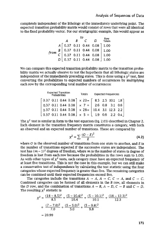
to the fixed probability vector. For our stratigraphic example, this would appear as
to Row
A B C D Totals
A 0.37 0.11 0.44 0.08 1.00
B 0.37 0.11 0.44 0.08 1 .oo
from
C 0.37 0.11 0.44 0.08 1 .oo
D 0.37 0.11 0.44 0.08 1 .oo

We can compare this expected transition probability matrix to the transition proba-
bility matrix we actually observe to test the hypothesis that all lithologic states are
independent of the immediately preceding states. This is done using a x2 test, first
converting the probabilities to expected numbers of occurrences by multiplying
each row by the corresponding total number of occurrences:

Expected Transition
Probabilities Totals Expected Frequencies
0.37 0.11 0.44 0.08 x 23= 8.5 2.5 10.1 1.8
0.37 0.11 0.44 0.08 x 7= 2.6 0.8 3.1 0.6
0.37 0.11 0.44 0.08 x 28= 10.4 3.1 12.3 2.2
0.37 0.11 0.44 0.08 x 5= 1.9 0.6 2.2 0.4
The x2 test is similar in form to the test equation (Eq. 2.65) described in Chapter 2.
Each element in the transition frequency matrix constitutes a category, with both
an observed and an expected number of transitions. These are compared by
(0 - E)'
x2=c c
I;
where 0 is the observed number of transitions from one state to another, and E is
the number of transitions expected if the successive states are independent. The
test has (m - 1)' degrees of freedom, where m is the number of states (a degree of
freedom is lost from each row because the probabilities in the rows sum to 1.00).
As with other types of x2 tests, each category must have an expected frequency of
at least five transitions. This is not the case in this example, but we can still make
a conservative test of independence by calculating the test statistic using the four
categories whose expected frequency is greater than five. The remaining categories
can be combined until their expected frequencies exceed five.
The categories include the transitions A - A, A - C, C - A, and C - C.
Combined categories can be formed of all elements in the B row, all elements in
the D row, and the combination of transitions A - B, A - D, C - B and C - D.
The resulting x2 statistic is

2 - (18 - 8.5)' + (5 - 10.4)' + (5 - 10.1)' + (18 - 12.3)'
- 8.5 10.4 10.1 12.3
(7 - 7.0)' + (5 - 5.0)' + (5 - 9.8)'
+ 7.0 5.0 9.8
= 20.99

171