Page 167 - Statistics and Data Analysis in Geology

Statistics and Data Analysis in Geology - Chapter 6

large. It is this tendency that allows us to use the normal probability distribution as
a basis for statistical tests and provides the starting point for the development of
the t-, F-, and x2 distributions and others. The concept of the normal distribution
can be extended to include situations in which observational units consist of many
variables.
Suppose we collect rocks from an area and measure a set of properties on each
specimen. The measurements may include determinations of chemical or miner-
alogical constituents, specific gravity, magnetic susceptibility, radioactivity, or any
of an almost endless list of possible variables. We can regard the set of measure-
ments made on an individual rock as defining a vector Xi = [ xli x~i - - xmi ],
s
where there are m measured characteristics or variables. If a sample of observa-
tions, each represented by vectors Xi, is randomly selected from a population that
is the result of many independently acting processes, the observed vectors will
tend to be multivariate normally distributed. Considered individually, each variate
is normally distributed and characterized by a mean, pj, and a variance, uj. The
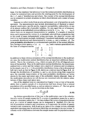
joint probabizity distribution is a p-dimensional equivalent of the normal distribu-
tion, having a vector mean p = [ p1 pz - . . pm ] and a variance generalized into
the form of a diagonal matrix:
u; 0 *-.
.
0 ::.. a& :1
.
1 0
In addition to these obvious extensions of the normal distribution to the multivari-
ate case, the multivariate normal distribution has an important additional charac-
teristic. This is the covariance, covjk, which occupies all of the off-diagonal posi-
tions of the matrixX. Thus, in the multivariate normal distribution, the mean is gen
eralized into a vector and the variance into a matrix of variances and covariances.
In the simple case of m = 2, the probability distribution forms a three-dimensional
bell curve such as that in Figure 2-19, shown as a contour map in Figure 6-4. Al-
though the distributions of variables x1 and x2 are shown along their respective
axes, the essential characteristics of the joint probability distribution are better
shown by the major and minor axes of the probability density ellipsoid. Many of
the multivariate procedures we will discuss are concerned with the relative orien-
tations of these major and minor axes.
One of the simplest tests we considered in Chapter 2 was a t-test of the prob-
ability that a random sample of n observations had been drawn from a normal
population with a specified mean, p, and an unknown variance, u2. The test, given
in Equation (2.45) on p. 70, can be rewritten in the form

(6.29)
An obvious generalization of this test to the multivariate case is the substitu-
tion of a vector of sample means for x, a vector of population means for p, and a
variance-covariance matrix for s2. We have defined the vector of population means
as p, so a vector of sample means can be designated X. Similarly, Z is the ma-
trix of population variances and covariances, so S represents the matrix of sample
variances and covariances. Both X and p are taken to be column vectors, although
equivalent equations may be written in which they are assumed to be row vectors. A
column vector of differences between the sample means and the population means

480