Page 168 - Statistics and Data Analysis in Geology

Analysis of Multivariate Data

-3
I I I I I I I I I I I
-5 -4 -3 -2 -1 0 1 2 3 4 5
XI
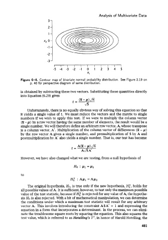
Figure 6-4. Contour map of bivariate normal probability distribution. See Figure 2.19 on
p. 40 for perspective diagram of same distribution.

is obtained by subtracting these two vectors. Substituting these quantities directly
into Equation (6.29) gives
(E -
t=
6

Unfortunately, there is no equally obvious way of solving this equation so that
it yields a single value of t. We must reduce the vectors and the matrix to single
numbers if we wish to apply this test. If we were to multiply the column vector
(E - p) by a row vector having the same number of elements, the result would be a
single number. We will therefore define an arbitrary row vector, A, whose transpose
is a column vector, A’. Multiplication of the column vector of differences (X - p)
by the row vector A gives a single number, and premultiplication of S by A and
postmultiplication by A’ also yields a single number. That is, our test has become

However, we have also changed what we are testing, from a null hypothesis of

to
H,* ApI =Ape

The original hypothesis, Ho, is true only if the new hypothesis, H,*, holds for
all possible values of A. It is sufficient, however, to test only the maximum possible
value of the test statistic, because if H,* is rejected for any value of A, the hypothe-
sis HO is also rejected. With a bit of mathematical manipulation, we can determine
the conditions under which a maximum test statistic will result for any arbitrary
vector A. This involves introducing the constraint ASA’ = 1 and expressing the
equation in a form that incorporates a determinant. In the process, we can elimi-
nate the troublesome square roots by squaring the equation. This also squares the
test value, which is referred to as Hotelling’s T2, in honor of Harold Hotelling, the

481