Page 163 - Statistics and Data Analysis in Geology

Statistics and Data Analysis in Geology - Chapter 6

I I I
1 1 ' 1 1 1 1 ' 1 ~ 1 1 ~ ~ 1 1 1 1 1 1 1 1 1 ~ ~ 1 ~ ~ 1 ~ 1
-335 -340 -345 -350 -355 -360 -365
Raw discriminant scores

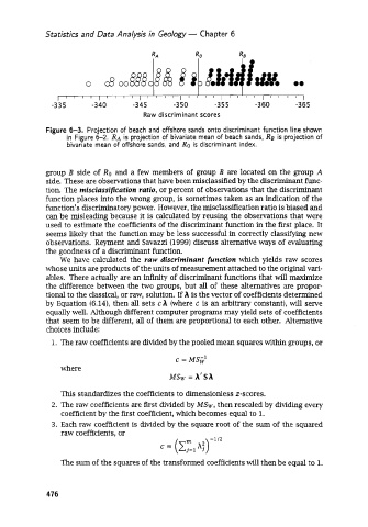
Figure 6-3. Projection of beach and offshore sands onto discriminant function line shown
in Figure 6-2. RA is projection of bivariate mean of beach sands, RB is projection of
bivariate mean of ofkhore sands, and Ro is discriminant index.

group B side of Ro and a few members of group B are located on the group A
side. These are observations that have been misclassified by the discriminant func-
tion. The misclassification ratio, or percent of observations that the discriminant
function places into the wrong group, is sometimes taken as an indication of the
function's discriminatory power. However, the misclassification ratio is biased and
can be misleading because it is calculated by reusing the observations that were
used to estimate the coefficients of the discriminant function in the first place. It
seems likely that the function may be less successful in correctly classifying new
observations. Reyment and Savazzi (1999) discuss alternative ways of evaluating
the goodness of a discriminant function.
We have calculated the YUW discriminant function which yields raw scores
whose units are products of the units of measurement attached to the original vari-
ables. There actually are an infinity of discriminant functions that will maximize
the difference between the two groups, but all of these alternatives are propor-
tional to the classical, or raw, solution. If A is the vector of coefficients determined
by Equation (6.14), then all sets cA (where c is an arbitrary constant), will serve
equally well. Although different computer programs may yield sets of coefficients
that seem to be different, all of them are proportional to each other. Alternative
choices include:

1. The raw coefficients are divided by the pooled mean squares within groups, or

c = MSK'
where
MSw = A'SA
This standardizes the coefficients to dimensionless z-scores.
2. The raw coefficients are first divided by MSw, then rescaled by dividing every
coefficient by the first coefficient, which becomes equal to 1.
3. Each raw coefficient is divided by the square root of the sum of the squared
raw coefficients. or

The sum of the squares of the transformed coefficients will then be equal to 1.

476