Page 40 - Statistics and Data Analysis in Geology

Elementary Statistics

rather, we will observe a continuous distribution of possible values. This is a fun-
damental characteristic of a continuous random variable.
To further illustrate the nature of a continuous random variable, we can con-
sider the problem of performing permeability tests on core samples. Permeabilities
are determined by measuring the time required to force a certain amount of fluid,
under standardized conditions, through a piece of rock. Suppose one test indi-
cates a permeability of 108 md (millidarcies). Is this the “true” permeability of the
sample? A second test run on the same specimen may yield a permeability of 93
md, and a third test may register 112 md. The permeability that is recorded on
the instruments during any given run is affected by conditions which inevitably
vary within the instrument from test to test, vagaries of flow and turbulence that
occur within the sample, and inconsistencies in the performance of the test by the
operator. No single test can be taken as an exactly correct measure of the true
permeability. The various sources of fluctuation combine to yield a continuously
random variable, which we are sampling by making repeated measurements.
Variation induced into measurements by inaccuracy of instrumentation is most
apparent when repeated measurements are made on a single object or a test is
repeated without change. This variation is called experimental emor. In contrast,
variation may occur between members of a set if measurements or experiments
are performed on a series of test objects. This is usually the variation that is of
scientific interest. Sometimes the two types of variations are hopelessly mixed
together, or confounded, and the experimenter cannot determine what portion of
the variability is due to variation between his test objects and what is due to error.
Rather than a single piece of rock, suppose we have a sizable length of core
taken from a borehole through a sandstone body. We want to determine the per-
meability of the sandstone, but obviously cannot put 20 ft of core into our per-
meability apparatus. Instead, we cut small plugs from the larger core at intervals
and determine the permeability of each. The variation we see is due in part to dif-
ferences between the test plugs, but also results from differences in experimental
conditions. Devising methods to estimate the magnitude of different sources of
variation is one of the major tasks of statistics.
Repeated measurements on large samples drawn from natural populations may
produce a characteristic frequency distribution. Most values are clustered around
some central value, and the frequency of occurrence declines away from this central
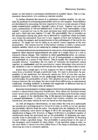
point. A graph of the distribution (Fig. 2-10) appears bell-shaped, and is called
a normal distribution. It often is assumed that random variables are normally
distributed, and many statistical tests are based on this supposition.
As with all frequency distributions, we may define the total area underneath
the normal curve as being equal to 1.00 (or if we wish, as loo%), so we can calculate
the probability directly from the curve. You should note the similarity of the bell-
shaped continuous curve shown in Figure 2-10 to the histogram of the binomial
distribution in Figure 2-9. However, in Figure 2-10 there is an infinite number of
subdivisions along the horizontal axis so the probability of obtaining one exact,
specific event is essentially zero. Instead, we consider the probability of obtaining
a result within a specified range. This probability is proportional to the area of
the frequency curve bounded by these limits. If our specified range is wide, we
are more likely to observe an event within them; if the range is extremely narrow,
observing an event is extremely unlikely.

27