Page 75 - Statistics and Data Analysis in Geology

Matrix Algebra

five elements, corrected for their means. If we divide a corrected sum of squares
by n - 1 we obtain the variance, and if we divide a corrected sum of products by
n - 1 we obtain the covariance. These are the elements of the covariance matrix, S,
which we can compute by
s = (n - i1-l~~~
A subset of S could serve our purposes (and the covariance matrix often is
used in multivariate statistics), but the relationships will be clearer if we use the
correlation matrix, R. Correlations are simply covariances of standardized variables;
that is, observations from which the means have been removed and then divided
by the standard deviation. In matrix D, the means have already been removed. We
can, in effect, divide by the appropriate standard deviations if we create a 5 x 5
matrix, C, whose diagonal elements are the square roots of the variances found on
the diagonal of S, and whose off-diagonal elements are all 0.0. If we invert C and
premultiply by D, each element of D will be divided by the standard deviation of its
column. Call the result U, a 20 x 5 matrix of standardized values;

U = DC-’

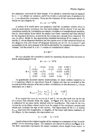
We can calculate the correlation matrix by repeating the procedure we used to
find S, substituting U for D:
R = (n - l)-lUTU

1 -0.312 0.141 0.85 0.595
-0.312 1 -0.201 -0.33 -0.28 1
R = 0.141 -0.201 1 -0.029 0.456
0.85 -0.33 -0.029 1 0.242
1 0.595 -0.28 0.456 0.242 1
To graphically illustrate matrix relationships, we must confine ourselves to
2 x 2 matrices, which we can extract from R. Copper and zinc are recorded in the
second and fifth columns of M, and so their correlations are the elements Yi,j whose
subscripts are 2 and 5:

= [ 1 -0.28
Rcu,,.,, = [ Y212 “g5] 1
r5,2 r5,S -0.28 1

If we regard the rows as vectors in X and Y, we can plot each row as the tip
of a vector that extends from the origin. In Figure 3-1, the tip of each vector
is indicated by an open circle, labeled with its coordmates. The ends of the two
vectors lie on an ellipse whose center is at the origin of the coordinate system and
which just encloses the tips of the vectors. The eigenvalues of the 2 x 2 matrix
R,,,,, represent the magnitudes, or lengths, of the major and minor semiaxes of
the ellipse. In this example, the eigenvalues are

hi = 1.28 A2 = 0.72

Gould refers to the relative lengths of the semiaxes as a measure of the “stretch-
ability” of the enclosing ellipse. The semiaxes are shown by arrows on Figure 3-1.
The first eigenvalue represents the major semiaxis whose length from center to

147