Page 80 - Statistics and Data Analysis in Geology

Statistics and Data Analysis in Geology - Chapter 3

Each eigenvector can be regarded as a set of coordinates in five-dimensional
space that defines the “direction” of a semiaxis of a hyperellipsoid. The length of
each semiaxis is given by the corresponding eigenvalue. The first semiaxis is twice
as long as the second, which is almost twice the length of the third. The fourth
axis is very short, and the fifth axis is almost nonexistent; the hyperellipse defined
by the correlation matrix, R, is really only a three-dimensional disk embedded in a
space of five dimensions.

The slope of a line drawn from the origin of a graph through a point is defined
by the ratio between the two coordinates of the point, and not by the actual mag-
nitudes of the coordinates. Similarly, the absolute magnitudes of the elements in
eigenvectors are not significant, only the ratios between the elements. An eigen-
vector can be scaled by multiplying by any arbitrary constant, and it will still define
the same direction in multidimensional space. Different computer programs may
return different eigenvectors for the same matrix; the eigenvectors simply have
been scaled in different ways. Most programs normalize, or scale each eigenvector
so the sum of the squares of each element in a vector will be equal to 1.0. Others
scale each eigenvector so the sum of its elements will be equal to its eigenvalue.
Although such results appear to be different, the ratios between pairs of elements
in the eigenvectors remain the same, and the vectors they define point in the same
“direction.” Also, you may note that the pattern of signs on the elements of the
eigenvectors seems to be different for two otherwise identical sets of eigenvectors.
This merely means that one set of vectors has been multiplied by (-l), reversing
its “direction” but not changing its orientation in multivariate space.
Increasingly, computer programs for multivariate analysis employ alternative
techniques for obtaining eigenvalues and eigenvectors. Rather than reducing a rect-
angular data matrix to a symmetrical, square correlation or covariance matrix and
then extracting the desired eigenvalues and eigenvectors as we have done, these
programs obtain results directly from the data matrix by singular value decom-
position (SVD). An excellent description of SVD is given by Jackson (1991); Press
and others (1992) provide a more compact presentation, as well as computer pro-
gram listings. We will delay a discussion of this procedure until Chapter 6, where
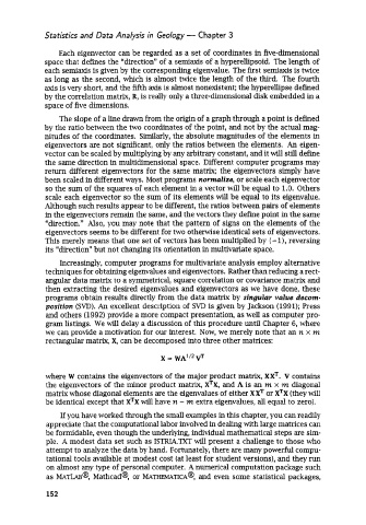
we can provide a motivation for our interest. Now, we merely note that an n x m
rectangular matrix, X, can be decomposed into three other matrices:

where W contains the eigenvectors of the major product matrix, XXT. V contains
the eigenvectors of the minor product matrix, XTX, and A is an m x m diagonal
matrix whose diagonal elements are the eigenvalues of either XXT or XTX (they will
be identical except that XTX will have n - m extra eigenvalues, all equal to zero).
If you have worked through the small examples in this chapter, you can readily
appreciate that the computational labor involved in dealing with large matrices can
be formidable, even though the underlying, individual mathematical steps are sim-
ple. A modest data set such as 1STRIA.m will present a challenge to those who
attempt to analyze the data by hand. Fortunately, there are many powerful compu-
tational tools available at modest cost (at least for student versions), and they run
on almost any type of personal computer. A numerical computation package such
as MATLAB@, Mathcad@, or MATHEMATICA@, and even some statistical packages,

152