Page 181 - Statistics for Dummies

165
Chapter 11: Sampling Distributions and the Central Limit Theorem

to denote actual outcomes of random variables. A distribution is a listing,
graph, or function of all possible outcomes of a random variable (such as X)
and how often each actual outcome (x), or set of outcomes, occurs. (See
Chapter 8 for more details on random variables and distributions.) 30

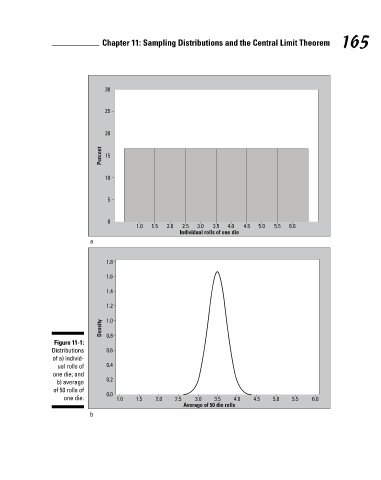
For example, suppose a million of your closest friends each rolls a single die
and records each actual outcome (x). A table or graph of all these possible 25
outcomes (one through six) and how often they occurred represents the
distribution of the random variable X. A graph of the distribution of X in this 20
case is shown in Figure 11-1a. It shows the numbers 1–6 appearing with equal
frequency (each one occurring ⁄6 of the time), which is what you expect over
1
many rolls if the die is fair. Percent 15
Now suppose each of your friends rolls this single die 50 times (n = 50) and
records the average, . The graph of all their averages of all their samples 10
represents the distribution of the random variable . Because this distribu-
tion is based on sample averages rather than individual outcomes, this distri-
bution has a special name. It’s called the sampling distribution of the sample 5
mean, . Figure 11-1b shows the sampling distribution of , the average of
50 rolls of a die. 0
1.0 1.5 2.0 2.5 3.0 3.5 4.0 4.5 5.0 5.5 6.0
Individual rolls of one die
Figure 11-1b (average of 50 rolls) shows the same range (1 through 6) of out-
comes as Figure 11-1a (individual rolls), but Figure 11-1b has more possible a
outcomes. You could get an average of 3.3 or 2.8 or 3.9 for 50 rolls, for exam-
ple, whereas someone rolling a single die can only get whole numbers from 1.8
1 to 6. Also, the shape of the graphs are different; Figure 11-1a shows a flat
shape, where each outcome is equally likely, and Figure 11-1b has a mound 1.6
shape; that is, outcomes near the center (3.5) occur with high frequency and
outcomes near the edges (1 and 6) occur with extremely low frequency. A 1.4
detailed look at the differences and similarities in shape, center, and spread
for individuals versus averages, and the reasons behind them, is the topic of 1.2
the following sections. (See Chapter 8 if you need background info on shape,
Density
center, and spread of random variables before diving in.) 1.0
Figure 11-1: 0.8
The Mean of a Sampling Distribution Distributions 0.6
of a) individ-
ual rolls of 0.4
Using the die-rolling example from the preceding section, X is a random vari- one die; and
able denoting the outcome you can get from a single die (assuming the die b) average 0.2
is fair). The mean of X (over all possible outcomes) is denoted by (pro- of 50 rolls of
nounced mu sub-x); in this case its value is 3.5 (as shown in Figure 11-1a). If one die. 0.0 1.0 1.5 2.0 2.5 3.0 3.5 4.0 4.5 5.0 5.5 6.0
you roll a die 50 times and take the average, the random variable repre- Average of 50 die rolls
sents any outcome you could get. The mean of , denoted (pronounced b
mu sub-x-bar) equals 3.5 as well. (You can see this result in Figure 11-1b.)

17_9780470911082-ch11.indd 165 3/25/11 10:01 PM