Page 183 - Statistics for Dummies

167
Chapter 11: Sampling Distributions and the Central Limit Theorem

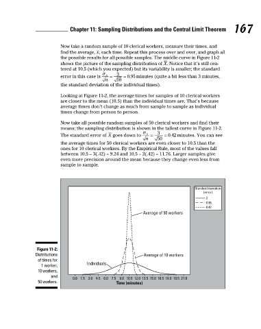
This result is no coincidence! In general, the mean of the population of all Now take a random sample of 10 clerical workers, measure their times, and
possible sample means is the same as the mean of the original population. find the average, , each time. Repeat this process over and over, and graph all
(Notationally speaking, you write .) It’s a mouthful, but it makes sense the possible results for all possible samples. The middle curve in Figure 11-2
that the average of the averages from all possible samples is the same as shows the picture of the sampling distribution of . Notice that it’s still cen-
the average of the population that the samples came from. In the die rolling tered at 10.5 (which you expected) but its variability is smaller; the standard
example, the average of the population of all 50-roll averages equals the aver- error in this case is minutes (quite a bit less than 3 minutes,
age of the population of all single rolls (3.5).
the standard deviation of the individual times).
Using subscripts on , you can distinguish which mean you’re talking
about — the mean of X (all individuals in a population) or the mean of Looking at Figure 11-2, the average times for samples of 10 clerical workers
(all sample means from the population). are closer to the mean (10.5) than the individual times are. That’s because
average times don’t change as much from sample to sample as individual
times change from person to person.
Measuring Standard Error Now take all possible random samples of 50 clerical workers and find their
means; the sampling distribution is shown in the tallest curve in Figure 11-2.

The values in any population deviate from their mean; for instance, people’s The standard error of goes down to minutes. You can see
heights differ from the overall average height. Variability in a population of the average times for 50 clerical workers are even closer to 10.5 than the
individuals (X) is measured in standard deviations (see Chapter 5 for details ones for 10 clerical workers. By the Empirical Rule, most of the values fall
on standard deviation). Sample means vary because you’re not sampling the between 10.5 – 3(.42) = 9.24 and 10.5 + 3(.42) = 11.76. Larger samples give
whole population, only a subset; and as samples vary, so will their means. even more precision around the mean because they change even less from
Variability in the sample mean ( ) is measured in terms of standard errors. sample to sample.
Error here doesn’t mean there’s been a mistake — it means there is a gap
between the population and sample results.
Standard deviation
The standard error of the sample mean is denoted by (sigma sub-x-bar). Its (error)
formula is , where is population standard deviation (sigma sub-x) and 3
0.95
n is size of each sample. In the next sections you see the effect each of these 0.42
two components has on the standard error. Average of 50 workers

Sample size and standard error

The first component of standard error is the sample size, n. Because n is in
the denominator of the standard error formula, the standard error decreases Figure 11-2:
as n increases. It makes sense that having more data gives less variation (and Distributions Average of 10 workers
more precision) in your results. of times for
1 worker, Individuals
Suppose X is the time it takes for a clerical worker to type and send one letter of 10 workers,
recommendation, and say X has a normal distribution with mean 10.5 minutes and 0.0 1.5 3.0 4.5 6.0 7.5 9.0 10.5 12.0 13.5 15.0 16.5 18.0 19.5 21.0
and standard deviation 3 minutes. The bottom curve in Figure 11-2 shows the 50 workers. Time (minutes)

picture of the distribution of X, the individual times for all clerical workers in the
population. According to the Empirical Rule (see Chapter 9), most of the values
are within 3 standard deviations of the mean (10.5) — between 1.5 and 19.5.

17_9780470911082-ch11.indd 167 3/25/11 10:01 PM