Page 180 - Statistics for Dummies

164 Part III: Distributions and the Central Limit Theorem

to denote actual outcomes of random variables. A distribution is a listing,
graph, or function of all possible outcomes of a random variable (such as X)
and how often each actual outcome (x), or set of outcomes, occurs. (See
Chapter 8 for more details on random variables and distributions.)

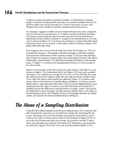
For example, suppose a million of your closest friends each rolls a single die
and records each actual outcome (x). A table or graph of all these possible
outcomes (one through six) and how often they occurred represents the
distribution of the random variable X. A graph of the distribution of X in this
case is shown in Figure 11-1a. It shows the numbers 1–6 appearing with equal
frequency (each one occurring ⁄6 of the time), which is what you expect over
1
many rolls if the die is fair.
Now suppose each of your friends rolls this single die 50 times (n = 50) and
records the average, . The graph of all their averages of all their samples
represents the distribution of the random variable . Because this distribu-
tion is based on sample averages rather than individual outcomes, this distri-
bution has a special name. It’s called the sampling distribution of the sample
mean, . Figure 11-1b shows the sampling distribution of , the average of
50 rolls of a die.

Figure 11-1b (average of 50 rolls) shows the same range (1 through 6) of out-
comes as Figure 11-1a (individual rolls), but Figure 11-1b has more possible
outcomes. You could get an average of 3.3 or 2.8 or 3.9 for 50 rolls, for exam-
ple, whereas someone rolling a single die can only get whole numbers from
1 to 6. Also, the shape of the graphs are different; Figure 11-1a shows a flat
shape, where each outcome is equally likely, and Figure 11-1b has a mound
shape; that is, outcomes near the center (3.5) occur with high frequency and
outcomes near the edges (1 and 6) occur with extremely low frequency. A
detailed look at the differences and similarities in shape, center, and spread
for individuals versus averages, and the reasons behind them, is the topic of
the following sections. (See Chapter 8 if you need background info on shape,
center, and spread of random variables before diving in.)

The Mean of a Sampling Distribution

Using the die-rolling example from the preceding section, X is a random vari-
able denoting the outcome you can get from a single die (assuming the die
is fair). The mean of X (over all possible outcomes) is denoted by (pro-
nounced mu sub-x); in this case its value is 3.5 (as shown in Figure 11-1a). If
you roll a die 50 times and take the average, the random variable repre-
sents any outcome you could get. The mean of , denoted (pronounced
mu sub-x-bar) equals 3.5 as well. (You can see this result in Figure 11-1b.)

17_9780470911082-ch11.indd 164 3/25/11 10:01 PM