Page 182 - Statistics for Environmental Engineers

L1592_frame_C21 Page 181 Tuesday, December 18, 2001 2:43 PM

Case Study: Water Quality Compliance
A company is required to meet a water quality limit of 300 ppm in a river. This has been monitored by
collecting specimens of river water during the first week of each of the past 27 quarters. The data are
from Hahn and Meeker (1991).

48 94 112 44 93 198 43 52 35
170 25 22 44 16 139 92 26 116
91 113 14 50 75 66 43 10 83

There have been no violations so far, but the company wants to use the past data to estimate the probability
that a future quarterly reading will exceed the regulatory limit of L = 300.
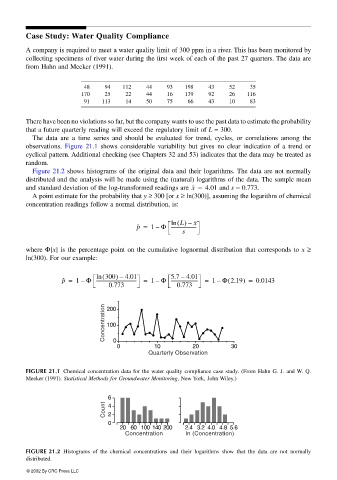
The data are a time series and should be evaluated for trend, cycles, or correlations among the
observations. Figure 21.1 shows considerable variability but gives no clear indication of a trend or
cyclical pattern. Additional checking (see Chapters 32 and 53) indicates that the data may be treated as
random.
Figure 21.2 shows histograms of the original data and their logarithms. The data are not normally
distributed and the analysis will be made using the (natural) logarithms of the data. The sample mean
and standard deviation of the log-transformed readings are x = 4.01 and s = 0.773.
A point estimate for the probability that y ≥ 300 [or x ≥ ln(300)], assuming the logarithm of chemical
concentration readings follow a normal distribution, is:

ln
L () –
p ˆ = 1 Φ ---------------------- x
–
s
where Φ[x] is the percentage point on the cumulative lognormal distribution that corresponds to x ≥
ln(300). For our example:

(
–
300) 4.01
–
5.7 4.01
ln
p ˆ = 1 Φ ------------------------------------ = 1 Φ ------------------------ = 1 Φ 2.19) = 0.0143
(
–
–
–
0.773 0.773
Concentration 200
100
0
0 10 20 30
Quarterly Observation
FIGURE 21.1 Chemical concentration data for the water quality compliance case study. (From Hahn G. J. and W. Q.
Meeker (1991). Statistical Methods for Groundwater Monitoring, New York, John Wiley.)

6
Count 4
2
0
20 60 100 140 200 2.4 3.2 4.0 4.8 5.6
Concentration In (Concentration)

FIGURE 21.2 Histograms of the chemical concentrations and their logarithms show that the data are not normally
distributed.
© 2002 By CRC Press LLC