Page 198 - The Combined Finite-Discrete Element Method

THE CENTRAL DIFFERENCE TIME INTEGRATION SCHEME 181

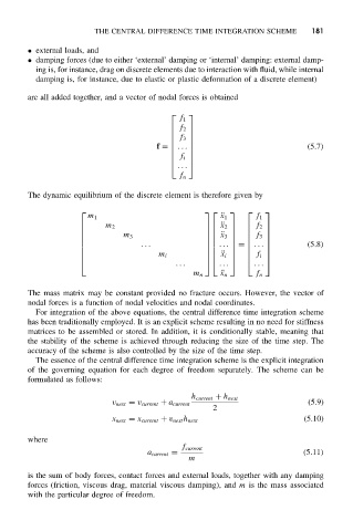
• external loads, and
• damping forces (due to either ‘external’ damping or ‘internal’ damping: external damp-
ing is, for instance, drag on discrete elements due to interaction with fluid, while internal
damping is, for instance, due to elastic or plastic deformation of a discrete element)

are all added together, and a vector of nodal forces is obtained

 
f 1
 f 2 
 
 f 3 
(5.7)
 
f =  .. . 
 
 f i 
.. .
 
f n
The dynamic equilibrium of the discrete element is therefore given by

     
m 1 ¨ x 1 f 1
m 2
   ¨x 2   f 2 
     
m 3
   ¨x 3   f 3 
... (5.8)
     
   ...  =  .. . 
     
m i
   ¨x i   f i 
... ... .. .
     
m n ¨ x n f n
The mass matrix may be constant provided no fracture occurs. However, the vector of
nodal forces is a function of nodal velocities and nodal coordinates.
For integration of the above equations, the central difference time integration scheme
has been traditionally employed. It is an explicit scheme resulting in no need for stiffness
matrices to be assembled or stored. In addition, it is conditionally stable, meaning that
the stability of the scheme is achieved through reducing the size of the time step. The
accuracy of the scheme is also controlled by the size of the time step.
The essence of the central difference time integration scheme is the explicit integration
of the governing equation for each degree of freedom separately. The scheme can be
formulated as follows:

h current + h next
v next = v current + a current (5.9)
2
x next = x current + v next h next (5.10)
where
f current
a current = (5.11)
m
is the sum of body forces, contact forces and external loads, together with any damping
forces (friction, viscous drag, material viscous damping), and m is the mass associated
with the particular degree of freedom.