Page 199 - The Combined Finite-Discrete Element Method

182 TEMPORAL DISCRETISATION

x next

x current

x prev
h next
h current

t current t next
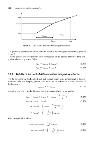
Figure 5.1 The central difference time integration scheme.

A graphical interpretation of the central difference time integration scheme is given in
Figure 5.1.
In the case of the constant time step, formulation of the central difference time inte-
gration scheme is given as follows:

v next = v current + a current h (5.12)
x next = x current + v next h (5.13)

5.1.1 Stability of the central difference time integration scheme

For the zero external load and internal and contact forces being proportional to the dis-
placement with no damping present, the force can be written as a linear function of
displacement:
f current =−kx current (5.14)
In such a case, the central difference time integration scheme is reduced to

kx current
v next = v current + a current h = v current − h (5.15)
m
x next = x current + v next h (5.16)

kx current 2
= v current h + x current − h
m
k

= v current h + 1 − h 2 x current
m
After multiplication with h

k 2
hv next = hv current − h x current (5.17)
m
k

x next = v current h + 1 − h 2 x current (5.18)
m