Page 202 - The Combined Finite-Discrete Element Method

DYNAMICS OF IRREGULAR DISCRETE ELEMENTS SUBJECT 185

5.2 DYNAMICS OF IRREGULAR DISCRETE ELEMENTS SUBJECT TO
FINITE ROTATIONS IN 3D

Very often a combined finite-discrete element system also comprises rigid discrete ele-
ments. In such cases, no forces due to deformation are present, while discretisation of
rigid discrete elements is necessary only for a description of the geometry of discrete ele-
ments and processing of contact interaction. In these types of problems, once the contact
forces and external loads are known, the governing equations can be integrated.
For systems comprising rigid bodies in 2D, in general this is achieved through solving
equations for translation and rotation about the centre of mass, i.e. assigning to each
discrete element three degrees of freedom – two translations in the direction of the coor-
dinate axes and one rotation about the z-axis. Thus, in 2D problems the central difference
time integration scheme as described in the previous section is directly applicable.
In 3D problems this situation is complicated by the presence of finite rotations about the
centre of mass of the discrete element. The problem with simply extending 2D algorithms
into 3D is that the angular velocity describing such rotation in general does not coincide
with the principal axes of the discrete element. Simple extension of 2D algorithms into 3D
would therefore not work. For instance, in 3D problems a description of spatial orientation
is not a trivial task.

5.2.1 Frames of reference

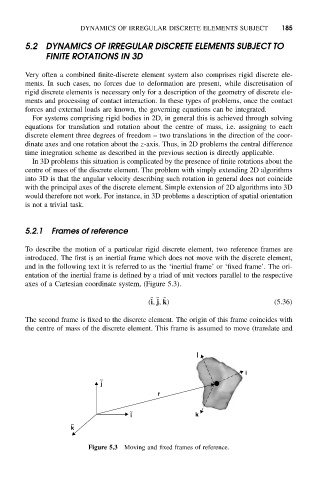
To describe the motion of a particular rigid discrete element, two reference frames are
introduced. The first is an inertial frame which does not move with the discrete element,
and in the following text it is referred to as the ‘inertial frame’ or ‘fixed frame’. The ori-
entation of the inertial frame is defined by a triad of unit vectors parallel to the respective
axes of a Cartesian coordinate system, (Figure 5.3).

˜ ˜ ˜
(i, j, k) (5.36)
The second frame is fixed to the discrete element. The origin of this frame coincides with
the centre of mass of the discrete element. This frame is assumed to move (translate and

j

i
~
j
r

~
i k
~
k

Figure 5.3 Moving and fixed frames of reference.