Page 208 - The Combined Finite-Discrete Element Method

DYNAMICS OF IRREGULAR DISCRETE ELEMENTS SUBJECT 191

ψ = hω
(5.67)
&
2 2 2
ψ = ψ + ψ + ψ
˜ x ˜ y ˜ z
while the rotated triad of unit vectors is as follows:

' (
(ψ · t i) (ψ · t i)
t+h i = 2 ψ + t i − 2 ψ cos(ψ) (5.68)
ψ ψ
1
+ (ψ × t i) sin(ψ)
ψ
' (
(ψ · t j) (ψ · t j)
t+h j = 2 ψ + t j − 2 ψ cos(ψ)
ψ ψ
1
+ (ψ × t j) sin(ψ)
ψ
' (
(ψ · t k) (ψ · t k)
t+h k = 2 ψ + t k − 2 ψ cos(ψ)
ψ ψ
1
+ (ψ × t k) sin(ψ)
ψ
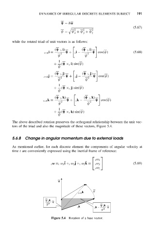
The above described rotation preserves the orthogonal relationship between the unit vec-
tors of the triad and also the magnitude of these vectors, Figure 5.4.

5.6.8 Change in angular momentum due to external loads

As mentioned earlier, for each discrete element the components of angular velocity at
time t are conveniently expressed using the inertial frame of reference:

 
t ω ˜x
˜ ˜ ˜
t ω = t ω ˜x i + t ω ˜y j + t ω ˜z k =  t ω ˜y  (5.69)
t ω ˜z

ψ

t +h k y

ψ k ψ
t
y 2 ψ k
t k t k − t ψ
y 2
Figure 5.4 Rotation of a base vector.