Page 209 - The Combined Finite-Discrete Element Method

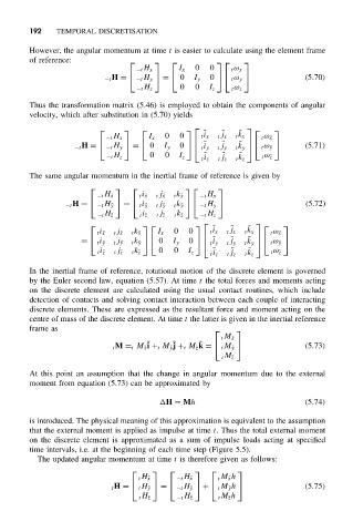
192 TEMPORAL DISCRETISATION

However, the angular momentum at time t is easier to calculate using the element frame
of reference:
     
0 0
−t H x I x t ω x
−t H =  −t H y  =  0 I y 0   t ω y  (5.70)
−t H z 0 0 I z t ω z
Thus the transformation matrix (5.46) is employed to obtain the components of angular
velocity, which after substitution in (5.70) yields
 
    ˜ ˜ ˜  
−t H x I x 0 0 t i x t j x t k x t ω ˜x
˜
˜

−t H =  −t H y  =  0 I y 0   ˜ t j y t k y   t ω ˜y  (5.71)
 t i y
−t H z 0 0 I z ˜ ˜ ˜ t ω ˜z
t i z t j z t k z
The same angular momentum in the inertial frame of reference is given by
     
−t H ˜x t i ˜x t j ˜x t k ˜x −t H x
−t H =  −t H ˜y  =  t i ˜y t j ˜y t k ˜y   −t H y  (5.72)
−t H ˜z t i ˜z t j ˜z t k ˜z −t H z
 
    ˜ ˜ ˜  
t i ˜x t j ˜x t k ˜x I x 0 0 t i x t j x t k x t ω ˜x
˜
˜

=  t i ˜y t j ˜y t k ˜y   0 I y 0   ˜ t j y t k y   t ω ˜y 
 t i y
t i ˜z t j ˜z t k ˜z 0 0 I z ˜ ˜ ˜ t ω ˜z
t i z t j z t k z
In the inertial frame of reference, rotational motion of the discrete element is governed
by the Euler second law, equation (5.57). At time t the total forces and moments acting
on the discrete element are calculated using the usual contact routines, which include
detection of contacts and solving contact interaction between each couple of interacting
discrete elements. These are expressed as the resultant force and moment acting on the
centre of mass of the discrete element. At time t the latter is given in the inertial reference
frame as
 
t M ˜x
˜ ˜ ˜ (5.73)
t M = t M ˜x i + t M ˜y j + t M ˜z k =  t M ˜y 
t M ˜z
At this point an assumption that the change in angular momentum due to the external
moment from equation (5.73) can be approximated by

H = Mh (5.74)

is introduced. The physical meaning of this approximation is equivalent to the assumption
that the external moment is applied as impulse at time t. Thus the total external moment
on the discrete element is approximated as a sum of impulse loads acting at specified
time intervals, i.e. at the beginning of each time step (Figure 5.5).
The updated angular momentum at time t is therefore given as follows:

     
t H ˜x −t H ˜x t M ˜x h
t H =  t H ˜y  =  −t H ˜y  +  t M ˜y h  (5.75)
t H ˜z −t H ˜z t M ˜z h