Page 214 - The Combined Finite-Discrete Element Method

DYNAMICS OF IRREGULAR DISCRETE ELEMENTS SUBJECT 197

and the spatial orientation of the discrete element at time t + h:
' (
(ψ · t i) (ψ · t i)
t+h i = 2 ψ + t i − 2 ψ cos(ψ) (5.91)
ψ ψ
1
+ (ψ × t i) sin(ψ)
ψ
' (
(ψ · t j) (ψ · t j)
t+h j = 2 ψ + t j − 2 ψ cos(ψ)
ψ ψ
1
+ (ψ × t j) sin(ψ)
ψ
' (
(ψ · t k) (ψ · t k)
t+h k = 2 ψ + t k − 2 ψ cos(ψ)
ψ ψ
1
+ (ψ × t k) sin(ψ)
ψ

Step 7: set

   
t ω ˜x t+h ω ˜x
t ω ˜y t+h ω ˜y
  =   (5.92)
t ω ˜z t+h ω ˜z
t i = t+h i (5.93)
t j = t+h j
t k = t+h k

t = t + h
and return to Step 1.
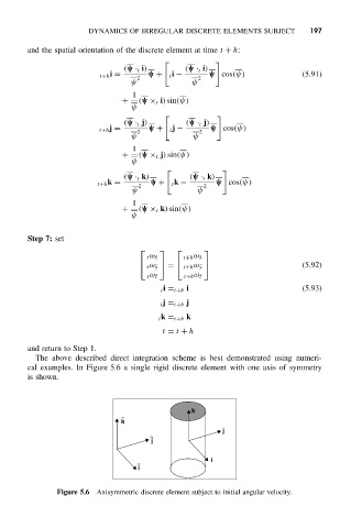
The above described direct integration scheme is best demonstrated using numeri-
cal examples. In Figure 5.6 a single rigid discrete element with one axis of symmetry
is shown.

k
~
k
j
~
j

i
~
i

Figure 5.6 Axisymmetric discrete element subject to initial angular velocity.