Page 211 - The Combined Finite-Discrete Element Method

194 TEMPORAL DISCRETISATION

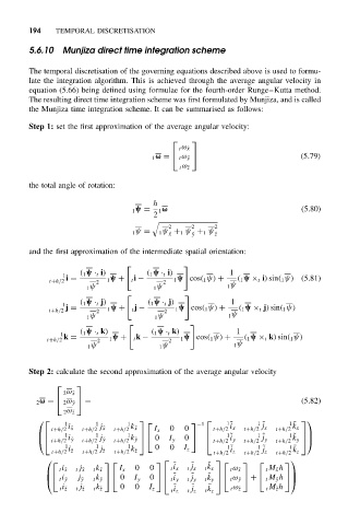
5.6.10 Munjiza direct time integration scheme

The temporal discretisation of the governing equations described above is used to formu-
late the integration algorithm. This is achieved through the average angular velocity in
equation (5.66) being defined using formulae for the fourth-order Runge–Kutta method.
The resulting direct time integration scheme was first formulated by Munjiza, and is called
the Munjiza time integration scheme. It can be summarised as follows:

Step 1: set the first approximation of the average angular velocity:

 
t ω ˜x
1 ω =  t ω ˜y  (5.79)
t ω ˜z

the total angle of rotation:

h
1 ψ = 1 ω (5.80)
2
&
2 2 2
1 ψ = 1 ψ + 1 ψ + 1 ψ ˜ z
˜ y
˜ x
and the first approximation of the intermediate spatial orientation:
' (
( 1 ψ · t i) ( 1 ψ · t i) 1
1
t+h/2 i = 2 1 ψ + t i − 2 1 ψ cos( 1 ψ) + ( 1 ψ × t i) sin( 1 ψ) (5.81)
1 ψ 1 ψ 1 ψ
' (
( 1 ψ · t j) ( 1 ψ · t j) 1
1
t+h/2 j = 2 1 ψ + t j − 2 1 ψ cos( 1 ψ) + ( 1 ψ × t j) sin( 1 ψ)
1 ψ 1 ψ 1 ψ
' (
( 1 ψ · t k) ( 1 ψ · t k) 1
1
t+h/2 k = 2 1 ψ + t k − 2 1 ψ cos( 1 ψ) + ( 1 ψ × t k) sin( 1 ψ)
1 ψ 1 ψ 1 ψ
Step 2: calculate the second approximation of the average angular velocity

 
2 ω ˜x
2 ω =  2 ω ˜y  = (5.82)
2 ω ˜z
1 1 1   −1 1 ˜ 1 ˜ 1 ˜
   
k
j
i
i
t+h/2 ˜x t+h/2 j ˜x t+h/2 k ˜x I x 0 0 t+h/2 x t+h/2 x t+h/2 x
1 1 1
j
 i   1 ˜ i 1 ˜ 1 ˜ k 
 t+h/2 ˜y t+h/2 j ˜y t+h/2 k ˜y   0 I y 0   t+h/2 y t+h/2 y t+h/2 y 
1 i 1 j 1 0 0 I z 1 ˜ 1 ˜ 1 ˜
i
k
j
t+h/2 ˜z t+h/2 ˜z t+h/2 k ˜z t+h/2 z t+h/2 z t+h/2 z
   
    ˜ ˜ ˜    
t i ˜x t j ˜x t k ˜x I x 0 0 t i x t j x t k x t ω ˜x t M ˜x h
  ˜ ˜ ˜  
 t i ˜y j ˜y t k ˜y   0 I y 0   t i y t j y  t ω ˜y  +  
 t k y  t M ˜y h 
t i ˜z t j ˜z t k ˜z 0 0 I z ˜ ˜ ˜ t ω ˜z t M ˜z h
t i z t j z t k z