Page 225 - The Combined Finite-Discrete Element Method

208 TEMPORAL DISCRETISATION

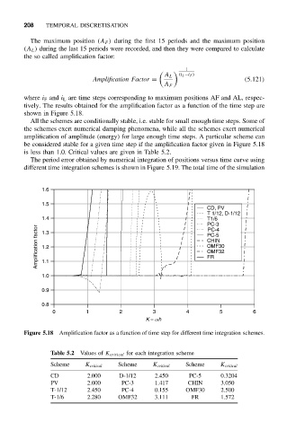
The maximum position (A F ) during the first 15 periods and the maximum position
(A L ) during the last 15 periods were recorded, and then they were compared to calculate
the so called amplification factor:

1

(i L −i F )
A L
Amplification Factor = (5.121)
A F
where i F and i L are time steps corresponding to maximum positions AF and AL, respec-
tively. The results obtained for the amplification factor as a function of the time step are
shown in Figure 5.18.
All the schemes are conditionally stable, i.e. stable for small enough time steps. Some of
the schemes exert numerical damping phenomena, while all the schemes exert numerical
amplification of amplitude (energy) for large enough time steps. A particular scheme can
be considered stable for a given time step if the amplification factor given in Figure 5.18
is less than 1.0. Critical values are given in Table 5.2.
The period error obtained by numerical integration of positions versus time curve using
different time integration schemes is shown in Figure 5.19. The total time of the simulation

1.6

1.5
CD, PV
T 1/12, D-1/12
1.4 T1/6
PC-3
Amplification factor 1.2 CHIN
PC-4
1.3
PC-5
OMF30
OMF32
FR
1.1
1.0

0.9
0.8
0 1 2 3 4 5 6
K = wh

Figure 5.18 Amplification factor as a function of time step for different time integration schemes.

Table 5.2 Values of K critical for each integration scheme
Scheme K critical Scheme K critical Scheme K critical
CD 2.000 D-1/12 2.450 PC-5 0.3204
PV 2.000 PC-3 1.417 CHIN 3.050
T-1/12 2.450 PC-4 0.155 OMF30 2.500
T-1/6 2.280 OMF32 3.111 FR 1.572