Page 226 - The Combined Finite-Discrete Element Method

ALTERNATIVE EXPLICIT TIME INTEGRATION SCHEMES 209

3.0
CD, PV T-1/6
D-1/12 PC-3
2.0 PC-4 PC-5
CHIN OMF30
OMF32 FR
1.0
Period error (%) after 1000 periods −1.0

0.0

−2.0

−3.0
0.0 0.2 0.4 0.6 0.8 1.0 1.2 1.4
K

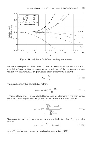
Figure 5.19 Period error for different time integration schemes.

was set to 1000 periods. The number of times that the curve crosses the x = 0 line is
recorded (n e ), and the time corresponding to the last time (t e ) the position curve crosses
the line x = 0 is recorded. The approximate period is calculated as shown:

2t e
T apr = (5.122)
n e
The period error is then calculated as follows:

(T apr − 2π)
ε period = 100 (5.123)
2π
The amplitude error is also evaluated from numerical integration of the position-time
curve for the one degree freedom by using the root mean square error formula:

)
i=n
*
(x − x exact )
* , 2
*
*
ε amplitude = 100 * i=1 % (5.124)
* i=n
x exact
,
+ 2
i=1
To separate the error in period from the error in amplitude, the value of x exact is calcu-
lated as
2π
x exact = sin t = sin ω apr t (5.125)
T apr
where T apr for a given time step is calculated using equation (5.122).