Page 318 - The Combined Finite-Discrete Element Method

POTENTIAL CONTACT FORCE IN 3D 301

.............continued from previous listing...........
for(i=0;i<nspoin;i++) /* intersection points */
{ inext=i+1; if(inext>=nspoin)inext=0;
for(j=0;j<3;j++)
{ jnext=j+1; if(jnext>2)jnext=0;
if((((dsc[i][j]>R0)&&(dsc[i][jnext]<R0))||
((dsc[i][j]<R0)&&(dsc[i][jnext]>R0)))&&
(((dcs[j][i]>R0)&&(dcs[j][inext]<R0))||
((dcs[j][i]<R0)&&(dcs[j][inext]>R0))))
{ factor=ABS(dsc[i][j]-dsc[i][jnext]);
if(factor<EPSILON){ factor=RP5; }
else { factor=ABS(dsc[i][j]/factor); }
ub[nbpoin]=(R1-factor)*uc[j]+factor*uc[jnext];
vb[nbpoin]=(R1-factor)*vc[j]+factor*vc[jnext];
nbpoin++;
}}}
for(i=1;i<nbpoin;i++)
{ if(vb[i]<vb[0])
{ tmp=vb[i]; vb[i]=vb[0]; vb[0]=tmp;
tmp=ub[i]; ub[i]=ub[0]; ub[0]=tmp;
}}
for(i=1;i<nbpoin;i++)
{ tmp=ub[i]-ub[0]; if(ABS(tmp)<EPSILON)tmp=EPSILON;
anb[i]=(vb[i]-vb[0])/tmp;
}
for(i=1;i<nbpoin;i++) /* sort B-points */
{ for(j=i+1;j<nbpoin;j++)
{ if(((anb[i]>=R0)&&(anb[j]>=R0)&&(anb[j]<anb[i]))||
((anb[i]<R0)&&((anb[j]>=R0)||(anb[j]<anb[i]))))
{ tmp=vb[i]; vb[i]=vb[j]; vb[j]=tmp;
tmp=ub[i]; ub[i]=ub[j]; ub[j]=tmp;
}}} }
if(nbpoin<3)continue;
/* Target-plain normal and penetration at B-points */
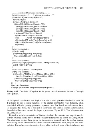
Listing 10.15 Calculation of B-points for the general case of intersection between a C-triangle
and S-polygon.

of the spatial coordinates, this implies that the contact potential distribution over the
B-polygon is also a linear function of the spatial coordinates. This function, when
multiplied with the penalty parameter, represents the distributed normal contact force.
To integrate this force, the B-polygon is subdivided into simplex shapes and integration
in analytical form over each of the shapes is performed (Figure 10.3). This is implemented
in Listing 10.17.
Equivalent nodal representation of this force for both the contactor and target tetrahedra
is then obtained. Nodal forces for the contactor tetrahedron are shown in Listing 10.18.
The distributed contact force acting on the contactor tetrahedron is the surface traction
force acting on the current surface of the contactor tetrahedron. Thus, only the tree nodes
defining this surface share the contact force, while the fourth node of the tetrahedron has