Page 71 - The Combined Finite-Discrete Element Method

54 PROCESSING OF CONTACT INTERACTION

3
B
2.99 A
Kinetic energy [GNm] 2.97 Legend
2.98

2.96
2.95
A
2.94
B
2.93
2.92
0 5 10 15 20 25
Time (ms)
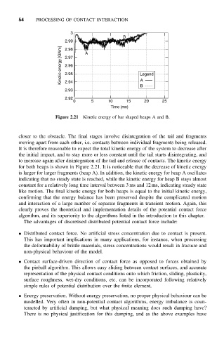
Figure 2.21 Kinetic energy of bar shaped heaps A and B.

closer to the obstacle. The final stages involve disintegration of the tail and fragments
moving apart from each other, i.e. contacts between individual fragments being released.
It is therefore reasonable to expect the total kinetic energy of the system to decrease after
the initial impact, and to stay more or less constant until the tail starts disintegrating, and
to increase again after disintegration of the tail and release of contacts. The kinetic energy
for both heaps is shown in Figure 2.21. It is noticeable that the decrease of kinetic energy
is larger for larger fragments (heap A). In addition, the kinetic energy for heap A oscillates
indicating that no steady state is reached, while the kinetic energy for heap B stays almost
constant for a relatively long time interval between 3 ms and 12 ms, indicating steady state
like motion. The final kinetic energy for both heaps is equal to the initial kinetic energy,
confirming that the energy balance has been preserved despite the complicated motion
and interaction of a large number of separate fragments in transient motion. Again, this
clearly proves the theoretical and implementation details of the potential contact force
algorithm, and its superiority to the algorithms listed in the introduction to this chapter.
The advantages of discretised distributed potential contact force include:

• Distributed contact force. No artificial stress concentration due to contact is present.
This has important implications in many applications, for instance, when processing
the deformability of brittle materials, stress concentrations would result in fracture and
non-physical behaviour of the model.
• Contact surface-driven direction of contact force as opposed to forces obtained by
the pinball algorithm. This allows easy sliding between contact surfaces, and accurate
representation of the physical contact conditions onto which friction, sliding, plasticity,
surface roughness, wet-dry conditions, etc. can be incorporated following relatively
simple rules of potential distribution over the finite element.
• Energy preservation. Without energy preservation, no proper physical behaviour can be
modelled. Very often in non-potential contact algorithms, energy imbalance is coun-
teracted by artificial damping, but what physical meaning does such damping have?
There is no physical justification for this damping, and as the above examples have