Page 73 - The Combined Finite-Discrete Element Method

56 PROCESSING OF CONTACT INTERACTION

closer the points to the contact surface, the greater the impact of the penetration. Thus,
the greatest error is at finite elements that are closest to the surface. In this way, the
maximum error introduced by the presence of penetration is a function of the maximum
allowed penetration, i.e. a function of element size. Since the maximum error due to the
finite element discretisation is also a function of element size, it implies that the same
mesh refinements will reduce both the error due to the finite element discretisation and
the error due to allowed penetration.

The main motivations behind the development of a potential contact force contact
algorithm are energy and momentum balance at finite penetrations. These must be achieved
by using a conventional in-core database for contact free finite element analysis.
The design of relational in-core databases for the contact free finite element analysis
has reached its maturity, and similar database designs can be found in most commercial
and academic codes. Most of the in-core databases are, to a large extent, normalised
to enable easy manipulation of the data with minimal storage requirements. This is to a
lesser extent valid for object orientated databases built mostly for object oriented codes or
distributed computing with parallel post-processing and visualisation facilities. However,
development in this direction is also expected to follow the logic of quick access and
minimum storage requirements.
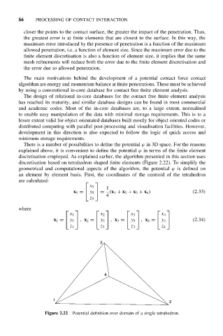
There is a number of possibilities to define the potential ϕ in 3D space. For the reasons
explained above, it is convenient to define the potential ϕ in terms of the finite element
discretisation employed. As explained earlier, the algorithm presented in this section uses
discretisation based on tetrahedron shaped finite elements (Figure 2.22). To simplify the
geometrical and computational aspects of the algorithm, the potential ϕ is defined on
an element by element basis. First, the coordinates of the centroid of the tetrahedron
are calculated:
 
x 5
1
x 5 =  y 5  = (x 1 + x 2 + x 3 + x 4 ) (2.33)
4
z 5
where
       
x 1 x 2 x 3 x 4
x 1 =  y 1  , x 2 =  y 2  , x 3 =  y 3  , x 4 =  y 4  (2.34)
z 1 z 2 z 3 z 4

3

4

1
2
Figure 2.22 Potential definition over domain of a single tetrahedron.