Page 262 - The Geological Interpretation of Well Logs

- THE GEOLOGICAL INTERPRETATION OF WELL LOGS -

NPHI GR

API

ray
Gamma

~«— main shale —_—— |
population

Neutron % —~
condensed
sequences
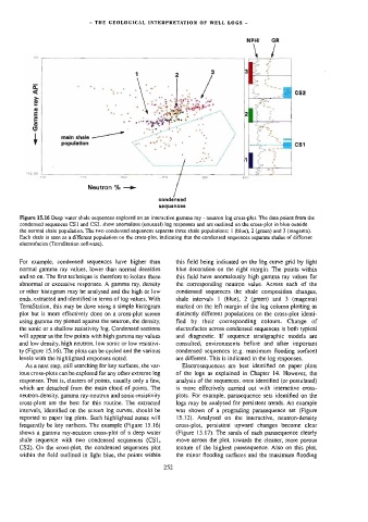
Figure 15.16 Deep water shale sequences explored on an interactive gamma ray - neutron log cross-plot. The data points from the
condensed sequences CS1 and CS2. show anomalous (unusual) log responses and are outlined on the cross-plot in blue outside
the normal shale population. The two condensed sequences separate three shale populations: | (blue), 2 (green) and 3 (magenta).
Each shale is seen as a different population on the cross-plot, indicating that the condensed sequences separate shales of different
electrofacies (TerraStation software).

For example, condensed sequences have higher than this field being indicated on the log curve grid by light
normal] gamma ray values, lower than normal densities blue decoration on the right margin. The points within
and so on. The first technique is therefore to isolate these this field have anomalously high gamma ray values for
abnormal or excessive responses. A gamma ray, density the cotresponding neutron value. Across each of the
or other histogram may be analysed and the high or low condensed sequences the shale composition changes,
ends, extracted and identified in terms of log values. With shale intervals 1 (blue), 2 (green) and 3 (magenta)
TerraStation, this may be done using a simple histogram marked on the left margin of the Jog column plotting as
plot but is more effectively done on a cross-plot screen distinctly different populations on the cross-plot identi-
using gamma ray piotted against the neutron, the density, fied by their corresponding colours. Change of
the sonic or a shallow resistivity log. Condensed sections electrofacies across condensed sequences is both typical
will appear as the few points with high gamma ray values and diagnostic. If sequence stratigraphic models are
and low density, high neutron, low sonic or low resistivi- consulted, environments before and after important
ty (Figure 15.16). The plots can be cycled and the various condensed sequences (e.g. maximum flooding surface)
levels with the highlighted responses noted. are different. This is indicated in the log responses.
As a next step, still searching for key surfaces, the var- Electrosequences are best identified on paper plots
ious cross-plots can be explored for any other extreme log of the logs as explained in Chapter 14. However, the
responses. That is, clusters of points, usually only a few, analysis of the sequences, once identified (or postulated)
which are detached from the main cloud of points. The is more effectively carried out with interactive cross-
neutron-density, gamma ray-neutron and sonic-resistivity plots. For example, parasequence sets identified on the
cross-plots are the best for this routine. The extracted logs may be analysed for persistent trends. An example
intervals, identified on the screen log curves, should be was shown of @ prograding parasequence set (Figure
reported to paper log plots. Such highlighted zones will 15.12). Analysed on the interactive, neutron-density
frequently be key surfaces. The example (Figure 15.16) cross-plot, persistent upward changes become clear
shows a gamma ray-neutron cross-plot of a deep water (Figure 15.17). The sands of each parasequence clearly
shale sequence with two condensed sequences (CS1, move across the plot, towards the cleaner, more porous
CS2). On the cross-plot, the condensed sequences plot texture of the highest parasequence. Also on this plot,
within the field outlined in light blue, the points within 252 the minor flooding surfaces and the maximum flooding