Page 180 - The Petroleum System From Source to Trap

172 Deming

° °
Temperature ( C) Temperature ( C)
20 40 60 80 1 00 1 4 0 0 40 80

1

2
'E 'E
.II: 2 .II:
+
.c .c · ·\ ·
+
.. .. +
D. D.
Cl)
Q)
c c
3 '\ + +
+ +
3
4

4
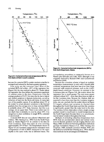
Figure 9.5. Corrected bottom-hole temperatures (BHTs)
from North Slope basin, Alaska.

extrapolation procedure is commonly known as a
Figure 9.4. Corrected bottom-hole temperatures (BHTs) Homer plot (Dowdle and Cobb, 197S), although it was
from Iberia oil field in south Louisiana. originally derived by Bullard (1947) and Lachenbruch
and Brewer (19S9).
because the corrected BHTs contain random noise that is Because this correction scheme is based on multiple
averaged and reduced by the least-squares regression. temperature measurements in each well, it should yield
How noisy are the corrected d a ta? Most of the corrected temperatures that have less error than those
corrected BHTs fall within ±10°C of the regression line corrected with empirical schemes, such as the AAPG
(Figure 9.4); the rms residual is about soc. Scatter about depth-based correction. However, in contrast to the
the regression line thus defines the maximum magnitude Louisiana data set (Figure 9.4), the scatter about the
of random noise in the data. Departures from the regression line is much greater. The root mean square
average gradient of 21.6°C/km may also be due to lateral residual is about 16°C-more than three times as high as
and vertical variations in thermal conductivity, as well as for the Louisiana data. Because the Alaskan data are
refraction of heat into the Iberia salt dome, to name just expected to have less error than the Louisiana tempera­
two of the possible reasons. If we attribute about 2°C of tures, one can conclude that the scatter shown in Figure
the scatter to actual physical variations in the thermal 9.S largely reflects real variation in thermal state
gradient, then the average error in these corrected BHTs throughout the North Slope basin and that this variation
is probably about ±S0C. Note, however, that this is an is significantly greater than the noise level in the data.
average, not an upper limit. There is one outlier near 2.4 The corollary to this observation is that a single average
km depth that is probably in error by about 30°C. It is gradient model is insufficient to model temperature in
dangerous to place confidence in single BHTs, corrected the North Slope basin because there is no accommoda­
or uncorrected. tion for lateral variation throughout the basin.
A second BHT data set was collected (Blanchard and Meth9ds of estimating subsurface temperature from
Tailleur, 1982; Deming et al., 1992) from the North Slope BHTs th'at can accommodate lateral and vertical varia­
basin in Alaska (Figure 9.5). In contrast to the data set tions in thermal gradients include kriging (Bodner and
from Louisiana, these data span an area covering Sharp, 1988), inversion for thermal gradients in individual
approximately 104-1()5 km2. The temperatures shown in geologic formations (Speece et al., 198S; Deming and
Figure 9.S are formation temperatures estimated from Chapman, 1988), stochastic inversion (Willett, 1990), and
extrapolation of sets of BHTs measured at the same the method of variable bias (Deming et al., 1990a). Each of
depths in the same wells, but at different times. The these methods has its advantages and limitations.