Page 104 - The Mechatronics Handbook

0066_Frame_C07 Page 14 Wednesday, January 9, 2002 3:39 PM

The balance of magnetic and elastic forces is then given by


1
1
NI
F = ---------Φ = --------- -------  2 = kd (7.35)
2
m 0 A m 0 A  ) 
R
or
2 2
( NI) 2 m 0 N I A
------------------------m 0 A = kd, ------------------------ = kd
(
4 d 0 – d) 2 4 d 0 –( d ) 2
2 2
(Note that the expression µ 0 N I has units of force.) Again as the current is increased, the total elastic
and electric stiffness goes to zero and one has the potential for buckling.

7.8 Dynamic Principles for Electric and Magnetic Circuits

The fundamental equations of electromagnetics stem from the work of nineteenth century scientists such
as Faraday, Henry, and Maxwell. They take the form of partial differential equations in terms of the field
quantities of electric field E and magnetic flux density B, and also involve volumetric measures of charge
density q and current density J (see, e.g., Jackson, 1968). Most practical devices, however, can be modeled
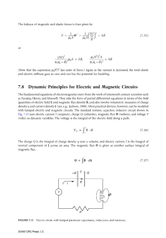
with lumped electric and magnetic circuits. The standard resistor, capacitor, inductor circuit shown in
Fig. 7.13 uses electric current I (amperes), charge Q (columbs), magnetic flux Φ (webers), and voltage V
(volts) as dynamic variables. The voltage is the integral of the electric field along a path:

⋅
V 21 = ∫ 2 E d l (7.36)
1
The charge Q is the integral of charge density q over a volume, and electric current I is the integral of
normal component of J across an area. The magnetic flux Φ is given as another surface integral of
magnetic flux.

Φ = ∫ B d A (7.37)
⋅

FIGURE 7.13 Electric circuit with lumped parameter capacitance, inductance, and resistance.

©2002 CRC Press LLC