Page 189 - The Mechatronics Handbook

0066_frame_C10 Page 9 Wednesday, January 9, 2002 4:10 PM

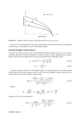
A O3 > A O2 > A O1

Cylinder Speed A O1 A O2 A O3

F max
External Load

FIGURE 10.4 Hydraulic cylinder load-speed relationship under the same system pressure.

Equation (10.27) indicates that the increase in speed stiffness can be achieved either by increasing the
system pressure or the cylinder size, or by decreasing the speed.

System Dynamic Characteristics
To analyze the dynamic characteristics of this hydraulic cylinder actuation system, one can use flow
continuity and system momentum equations to model the cylinder motion. Neglecting system leakage,
friction, and line loss, the following are the governing equations for the hydraulic system:

q = kx P P – P 1 = A 1 dy V 1 dP 1 (10.28)
----- +
----- --------
dt b dt
2
d y
P 1 A 1 = m -------- + F (10.29)
dt 2
To perform dynamic analysis on this hydraulic system, it is essential to derive its transfer function
based on the above nonlinear equation, which can be obtained by taking the Laplace transform on the
linearized form of the above equations (Watton, 1989).
 1 
----------dis() –  
V 1
k 1 K i ---------s + ------------- dFs()
2
2
A 1 A 1 b A 1 k 3 R o
dvs() = ---------------------------------------------------------------------------- (10.30)
1
2
---------ms + -------------ms + 1
V 1
2
2
A 1 b A 1 k 2 R o
Making
2
A 1 b
mb
1
w n = ----------, z = ------------- ------------, and K s = k 1 K i
----------
V 1 m 2k 2 R o V 1 A 1 2 A 1
Equation (10.30) can be represented as
1 

---- -----s + -------- d Fs()
1 V 1
K s dis() A 1 2  b k 3 R o 
dvs() = -------------------------------- – ----------------------------------------------- (10.31)
1
------s +
1
------s +
------s + 2z 1 ------s + 2z 1
2
2
2 2
w n w n w n w n
©2002 CRC Press LLC