Page 318 - The Mechatronics Handbook

0066_frame_C14.fm Page 32 Wednesday, January 9, 2002 1:51 PM

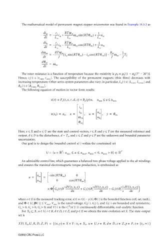
The mathematical model of permanent-magnet stepper micromotor was found in Example 14.5.3 as

1
------- = – ------i as + RTψ m ( RTθ rm ) + -----u as
di as
r s
--------------ω rm sin
dt L ss L ss L ss
1
------- = – ------i bs – RTψ m ( RTθ rm ) + -----u bs
di bs
r s
--------------ω rm cos
dt L ss L ss L ss
dω rm
RTψ m
----------- = – -------------- i as sin[ ( RTθ rm ) i bs cos ( RTθ rm )] – B m 1 --T L
------ω rm –
–
dt J J J
---------- = ω rm
dθ rm
dt
The rotor resistance is a function of temperature because the resistivity is ρ T = ρ 0 [(1 + α ρ (T° − 20°)].
Hence, r s (·) ∈[r s min r s max ]. The susceptibility of the permanent magnets (thin films) decreases with
increasing temperature. Other servo-system parameters also vary; in particular, L ss (·) ∈[L ss min L ss max ] and
B m (·) ∈[B m min B m max ].
The following equation of motion in vector form results:
x ˙ t() = F z t, x, r, d, z( ) + B p p()u, u min ≤ u ≤ u max

i as

xt 0 = x 0 , x = i bs , u = u as , y = θ rm
()
ω rm u bs
θ rm

Here, x ∈X and u ∈U are the state and control vectors, r ∈R and y ∈Y are the measured reference and
output, d ∈D is the disturbance, d = T L , and z ∈Z and p ∈P are the unknown and bounded parameter
uncertainties.
Our goal is to design the bounded control u(·) within the constrained set

2 2˙
U = {u ∈ : u min ≤ u ≤ u max , u min < 0, u max > 0} ⊂
An admissible control law, which guarantees a balanced two-phase voltage applied to the ab windings
and ensures the maximal electromagnetic torque production, is synthesized as

u = u as = – sin ( RTθ rm ) 0
0 cos ( RTθ rm )
u bs
)
T∂Vt, x, e(

× Φ G x t()B ------------------------- + G e t()B e T∂Vt, x, e( ∂e ) G i t()B e T1∂Vt, x, e( ∂e )  
------------------------- +
---------------------------

s
∂x
where e ∈E is the measured tracking error, e(t) = r(t) − y(t); Φ(·) is the bounded function (erf, sat, tanh),
and Φ ∈U, |Φ(·)| ≤ V max , V max is the rated voltage; G x (·), G e (·), and G i (·) are bounded and symmetric,
κ
G x > 0, G e > 0, G i > 0; and V(·) is the C (κ ≥ 1) continuously differentiable, real-analytic function.
For X 0 ⊆ , X u ∈U, r ∈R, d ∈D, z ∈Z, and p ∈P, we obtain the state evolution set X. The state-output
set is
(
XY X 0 ,U, R, D, Z, P) = ( { x, y) ∈ X × Y : x 0 ∈ X 0 , u ∈ U,r ∈ R, d ∈ D, z ∈ Z, p ∈ P, t ∈ [t 0 , ∞)}
©2002 CRC Press LLC