Page 317 - The Mechatronics Handbook

0066_frame_C14.fm Page 31 Friday, January 18, 2002 4:36 PM

and

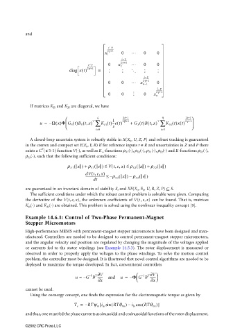
i−γ
-------------
2γ +1
x 1 0 L 0 0
i−γ
-------------
i−γ 0 2γ+1 L 0 0
------------- x 2
diag xt() 2γ+1 = M M O M M
i−γ
-------------
2γ +1
0 0 L x n−1 0
i−γ
-------------
0 0 M 0 x n 2γ+1
If matrices K Ei and K Xi are diagonal, we have

 ς ------------- η ------------- 
2i+1
2i+1
1
u = – Ω x()Φ G E t()B E t, x) T ∑ K Ei t()--et() 2β+1 + G X t()Bt, x) T ∑ K Xi t()xt() 2γ +1 
(
(

 s 
i=0 i=0
A closed-loop uncertain system is robustly stable in X(X 0 , U, Z, P) and robust tracking is guaranteed
in the convex and compact set E(E 0 , Y, R) if for reference inputs r ∈R and uncertainties in Z and P there
κ
exists a C (κ ≥ 1) function V(·), as well as K ∞ -functions ρ X1 (·), ρ X2 (·), ρ E1 (·), ρ E2 (·) and K-functions ρ X3 (·),
ρ E3 (·), such that the following sufficient conditions:
(
(
(
(
ρ X1 x ) + ρ E1 e ) ≤ Vt, e, x) ≤ ρ X2 x ) + ρ E2 e )
(
(
dV t, e, x) – ρ X3 x ) ρ E3 e )
(
(
------------------------- ≤
–
dt
are guaranteed in an invariant domain of stability S, and XE(X 0 , E 0 , U, R, Z, P) ⊆ S.
The sufficient conditions under which the robust control problem is solvable were given. Computing
the derivative of the V(t, e, x), the unknown coefficients of V(t , e, x) can be found. That is, matrices
K Ei (·) and K Xi (·) are obtained. This problem is solved using the nonlinear inequality concept [9].
Example 14.6.1: Control of Two-Phase Permanent-Magnet
Stepper Micromotors
High-performance MEMS with permanent-magnet stepper micromotors have been designed and man-
ufactured. Controllers are needed to be designed to control permanent-magnet stepper micromotors,
and the angular velocity and position are regulated by changing the magnitude of the voltages applied
or currents fed to the stator windings (see Example 14.5.3). The rotor displacement is measured or
observed in order to properly apply the voltages to the phase windings. To solve the motion control
problem, the controller must be designed. It is illustrated that novel control algorithms are needed to be
deployed to maximize the torque developed. In fact, conventional controllers
T∂V

T∂V
1
–
1
–
u = – G B ------- and u = – Φ G B -------- 

∂x ∂x 
cannot be used.
Using the coenergy concept, one finds the expression for the electromagnetic torque as given by
T e = – RTψ m i as sin ( RTθ rm ) i bs cos ( RTθ rm )]
[
–
and thus, one must fed the phase currents as sinusoidal and cosinusoidal functions of the rotor displacement.
©2002 CRC Press LLC