Page 369 - The Mechatronics Handbook

input terminals. High input impedance is desirable, since the device will then draw less current from the
source. Oscilloscopes and data acquisition equipment frequently have input impedances of 1 MΩ or
more to minimize this current draw. Output impedance is a measure of a sensor’s (or signal conditioning
circuit’s) ability to provide current for the next stage of the system. Output impedance is frequently
modeled as a resistor in series with the sensor output. Low output impedance is desirable, but is often
not available directly from a sensor. Piezoelectric sensors in particular have high output impedances and
cannot source much current (typically micro-amps or less). Op-amp circuits are frequently used to buffer
sensor outputs for this reason. Op-amp circuits (especially voltage followers) provide nearly ideal cir-
cumstances for many sensors, since they have high input impedance but can substantially lower output
impedance.

18.8 Nonlinearities

Linear systems have the property of superposition. If the response of the system to input A is output A,
and the response to input B is output B, then the response to input C (= input A + input B) will be
output C ( = output A + output B). Many real systems will exhibit linear or nearly linear behavior over
some range of operation. Therefore, linear system analysis is correct, at least over these portions of a
system’s operating envelope. Unfortunately, most real systems have nonlinearities that cause them to
operate outside of this linear region, and many common assumptions about system behavior, such as
superposition, no longer apply. Several nonlinearities commonly found in mechatronic systems include
static and coulomb friction, eccentricity, backlash (or hysteresis), saturation, and deadband.

18.9 Static and Coulomb Friction

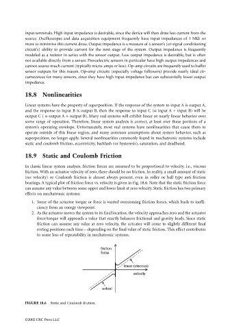
In classic linear system analysis, friction forces are assumed to be proportional to velocity, i.e., viscous
friction. With an actuator velocity of zero, there should be no friction. In reality, a small amount of static
(no velocity) or Coulomb friction is almost always present, even in roller or ball type anti-friction
bearings. A typical plot of friction force vs. velocity is given in Fig. 18.6. Note that the static friction force
can assume any value between some upper and lower limit at zero velocity. Static friction has two primary
effects on mechatronic systems:

1. Some of the actuator torque or force is wasted overcoming friction forces, which leads to ineffi-
ciency from an energy viewpoint.
2. As the actuator moves the system to its final location, the velocity approaches zero and the actuator
force/torque will approach a value that exactly balances frictional and gravity loads. Since static
friction can assume any value at zero velocity, the actuator will come to slightly different final
resting positions each time—depending on the final value of static friction. This effect contributes
to some loss of repeatability in mechatronic systems.

FIGURE 18.6 Static and Coulomb friction.

©2002 CRC Press LLC