Page 373 - The Mechatronics Handbook

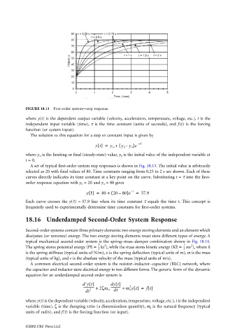
FIGURE 18.13 First-order system—step response.
where y(t) is the dependent output variable (velocity, acceleration, temperature, voltage, etc.), t is the
independent input variable (time), τ is the time constant (units of seconds), and f(t) is the forcing
function (or system input).
The solution to this equation for a step or constant input is given by
+
yt() = y ∞ ( y 0 y ∞ )e – t/t
–
where y ∞ is the limiting or final (steady-state) value, y 0 is the initial value of the independent variable at
t = 0.
A set of typical first-order system step responses is shown in Fig. 18.13. The initial value is arbitrarily
selected as 20 with final values of 80. Time constants ranging from 0.25 to 2 s are shown. Each of these
curves directly indicates its time constant at a key point on the curve. Substituting t = τ into the first-
order response equation with y 0 = 20 and y ∞ = 80 gives

– 1
–
y t() = 80 + ( 20 80)e = 57.9
Each curve crosses the y(τ) ≈ 57.9 line when its time constant τ equals the time t. This concept is
frequently used to experimentally determine time constants for first-order systems.

18.16 Underdamped Second-Order System Response

Second-order systems contain three primary elements: two energy storing elements and an element which
dissipates (or removes) energy. The two energy storing elements must store different types of energy. A
typical mechanical second-order system is the spring–mass–damper combination shown in Fig. 18.14.
1 2 1 2
--
--
The spring stores potential energy (PE = kx ), while the mass stores kinetic energy (KE = mv ), where k
2 2
is the spring stiffness (typical units of N/m), x is the spring deflection (typical units of m), m is the mass
(typical units of kg), and v is the absolute velocity of the mass (typical units of m/s).
A common electrical second-order system is the resistor–inductor–capacitor (RLC) network, where
the capacitor and inductor store electrical energy in two different forms. The generic form of the dynamic
equation for an underdamped second-order system is
2
d yt() dy t()
------------
------------- 2ζω n dt + ω n yt() = ft()
2
2 +
dt
where y(t) is the dependent variable (velocity, acceleration, temperature, voltage, etc.), t is the independent
variable (time), is the damping ratio (a dimensionless quantity), ω n is the natural frequency (typicalζ
units of rad/s), and f(t) is the forcing function (or input).

©2002 CRC Press LLC