Page 695 - The Mechatronics Handbook

0066_Frame_C23 Page 3 Wednesday, January 9, 2002 1:52 PM

be quite useful to classify the signals according to their energy or power content. The total energy over
the range t ∈(−∞, ∞) for a CT signal is given by

E = lim ∫ T/2 x t() d t (23.1)
2
T→∞ – T/2
and the average power is defined as
1
P = lim --- ∫ T/2 xt() d t (23.2)
2
T→∞ T – T/2
Consequently, x(t) is an energy signal if and only if 0 < E < ∞, which implies that P = 0. Similarly, x(t) is
a power signal if and only if 0 < P < ∞, indicating E = ∞. A signal that fails to satisfy either definition is,
therefore, neither energy nor power signal. These definitions are also applicable to DT signals except that the
integral in Eqs. (23.1) and (23.2) is replaced by summation. In general, periodic signals exist for all the
time and as such have infinite energy. However, they have finite average power, hence they are power
signals. On the other hand, bounded finite-duration signals are energy signals. The classification of a signal
to finite energy, finite power, or neither is important so that appropriate and effective procedures can be
selected for its analysis.
Singularity Functions
Singularity functions are useful for signal modeling, that is, they serve as basis for representing complex
signals to simplify their analysis.
The Unit Impulse Function
The impulse or delta function is a mathematical model for representing physical phenomena that occurs
within very small time duration; this time duration can be assumed to be equal to zero. The unit delta
function is not a mathematical function in the usual sense; rather it is a distribution or a generalized
function. Thus, the impulse function can be described by its effect on the test function φ(t), that is,
∫ +∞ φ t()δ t() t = φ 0() (23.3)
d
– ∞
provided φ(t) is continuous at t = 0. This equation shows the shifting property of the delta function. A
graphical plot of the delta function is shown in Fig. 23.3(a). Table 23.1 shows the operating properties
of the delta function.
The Unit Step Function
The unit step function is particularly useful for the mathematical analysis of CT signals. This is depicted
in Fig. 23.3(b), and is defined as

 1, t > 0
ut() =  (23.4)
 0, t < 0

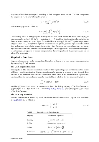
TABLE 23.1 Properties of the Delta Function
Property Mathematical Expression
+∞
(
d
Sampling ∫ xt()δ t – a) t = xa()
– ∞
(
Shifting xt()δ t –( a) = xa()δ t – a)

1
(
--
Scaling δ at ± b) ≡ -----δ t ± b 

a a
+∞
(
(
(
d
Convolution xt()∗δ t – a) = ∫ x τ()δ t τ – a) τ = xt – a)
–
– ∞
©2002 CRC Press LLC