Page 707 - The Mechatronics Handbook

0066_Frame_C23 Page 15 Wednesday, January 9, 2002 1:53 PM

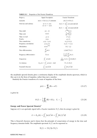
TABLE 23.5 Properties of the Fourier Transform
Property Signal Description Fourier Transform
Linearity ax t() + by t() ; a, b constants aX f() + bY f()
∞
t
Evenness and oddness x –() = xt() Xf() = 2 ∫ xt() cos ( 2πft) t
d
x –() = x – t() 0 ∞
t
Xf() = – 2 ∫ xt() sin ( 2πft) t
d
0
(
Time shift xt – t) e −j2πfτ X f()
f 
1
Time scale x at() -----X -- a 
a
∗
Time reversal x(−t) X ()
f
(
Duality X t() x – )
f
Time convolution x t() ∗ y t() X f() Y f()
Frequency convolution x t() y t() X f() ∗ Y f()
j2πf 0 t
(
Modulation xt()e X f – )
f 0
n
d
n
Time differentiation -------xt() ( j2pf ) Xf()
dt n
n
n
j  d
n
Frequency differentiation t x t()   ------ --------Xf()
2p
n
df
1
Integration ∫ ∞ x τ() τd ---------- Xf() + 1 --X 0()δ f()
– ∞ j2πf 2
(
–
d
Correlation R xy τ() = ∫ ∞ yt()xt τ) t Y –( f ) X f()
– ∞
2
2
Parseval’s theorem ∫ ∞ xt() d t ∫ ∞ Xf() d f
– ∞ – ∞
the amplitude spectral density gives a continuous display of the amplitude density spectrum, which in
this case is in the form of impulses, rather than just a number.
Similarly the Fourier transform of a train of impulses of the form
∞
(
pt() = ∑ δ tnT) (23.27)
–
n=∞
–
is given by
∞
1
Pf() = 1 ∑ δ fkF s ), F s = --- (23.28)
(
---
–
T T
k=∞
–
Energy and Power Spectral Density 6
Suppose x(t) is an aperiodic signal with a Fourier transform X( f ), then its energy is given by
2
E = R xx 0() = ∫ ∞ xt() d = ∫ ∞ Xf() d f (23.29)
2
t
– ∞ – ∞
This is Parseval’s theorem and it shows that the principle of conservation of energy in the time and
frequency domains holds. The amplitude spectrum X( f ) can be expressed as
Xf() = Xf() ∠ Xf()
©2002 CRC Press LLC