Page 749 - The Mechatronics Handbook

0066_Frame_C23 Page 57 Wednesday, January 9, 2002 1:56 PM

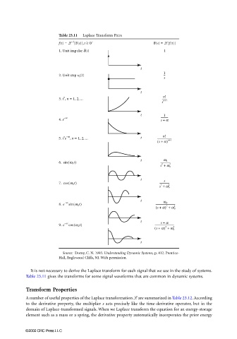
Table 23.11 Laplace Transform Pairs
f(t) = [F(s)],t ≥ 0 − F(s) = [f(t)]
−1
1. Unit impulse δ(t) 1

t
1
2. Unit step u s (t) --
s

t
n!
n
3. t , n = 1, 2, ... --------
s n+1
t 1
4. e −αt ------------
a
s +
n!
n −αt
5. t e , n = 1, 2, ... t -----------------------
( s + a) n+1

w 0
6. sin ( w 0 t) t ----------------
s + w 0 2
2
t s
7. cos ( w 0 t) ----------------
s + w 0 2
2
t
ω d
8. e – αt sin ( w d t) -------------------------------
2
( s + a) + w d 2
t s + a
9. e – αt cos ( w d t) -------------------------------
( s + a) + w d 2
2
t

Source: Dorny, C. N. 1993. Understanding Dynamic Systems, p. 412. Prentice-
Hall, Englewood Cliffs, NJ. With permission.

It is not necessary to derive the Laplace transform for each signal that we use in the study of systems.
Table 23.11 gives the transforms for some signal waveforms that are common in dynamic systems.

Transform Properties
A number of useful properties of the Laplace transformation are summarized in Table 23.12. According
to the derivative property, the multiplier s acts precisely like the time-derivative operator, but in the
domain of Laplace-transformed signals. When we Laplace transform the equation for an energy-storage
element such as a mass or a spring, the derivative property automatically incorporates the prior energy

©2002 CRC Press LLC