Page 745 - The Mechatronics Handbook

0066_Frame_C23 Page 53 Friday, January 18, 2002 5:35 PM

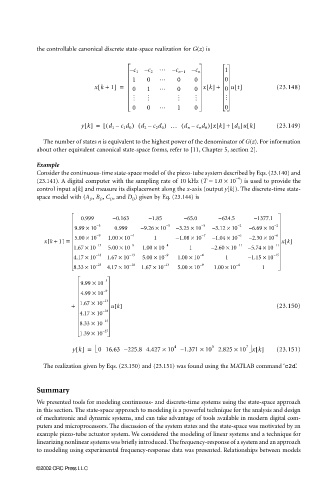
the controllable canonical discrete state-space realization for G(z) is

– c 1 – c 2 … – c n−1 – c n 1
1 0 … 0 0 0
[
xk + 1] = 0 1 … 0 0 xk[] + 0 ut[] (23.148)
M M M M M
0 0 … 1 0 0

yk[] = ( [ d 1 – c 1 d 0 ) ( d 2 – c 2 d 0 ) … ( d n – c n d 0 )]xk[] + []uk[] (23.149)
d 0
The number of states n is equivalent to the highest power of the denominator of G(z). For information
about other equivalent canonical state-space forms, refer to [11, Chapter 5, section 2].

Example
Consider the continuous-time state-space model of the piezo-tube system described by Eqs. (23.140) and
−4
(23.141). A digital computer with the sampling rate of 10 kHz (T = 1.0 × 10 ) is used to provide the
control input u[k] and measure its displacement along the x-axis (output y[k]). The discrete-time state-
space model with (A D , B D , C D , and D D ) given by Eq. (23.144) is

0.999 – 0.163 – 1.85 – 65.0 – 624.5 – 1377.1
9.99 × 10 – 5 0.999 – 9.26 × 10 – 5 – 3.25 × 10 – 3 – 3.12 × 10 – 2 – 6.69 × 10 – 2
5.00 × 10 – 9 1.00 × 10 – 4 1 −1.08 × 10 – 7 – 1.04 × 10 – 6 – 2.30 × 10 – 6
xk + 1] = xk[]
[
1.67 × 10 – 13 5.00 × 10 – 9 1.00 × 10 – 4 1 – 2.60 × 10 – 11 – 5.74 × 10 – 11
4.17 × 10 – 18 1.67 × 10 – 13 5.00 × 10 – 9 1.00 × 10 – 4 1 – 1.15 × 10 – 15
8.33 × 10 – 23 4.17 × 10 – 18 1.67 × 10 – 13 5.00 × 10 – 9 1.00 × 10 – 4 1
9.99 × 10 – 5
4.99 × 10 – 9

+ 1.67 × 10 – 13 uk[] (23.150)
4.17 × 10 – 18
8.33 × 10 – 23
1.39 × 10 – 27

5
7
4
yk[] = 0 16.63 – 225.8 4.427 × 10 – 1.371 × 10 2.825 × 10 xk[] (23.151)
The realization given by Eqs. (23.150) and (23.151) was found using the MATLAB command ‘c2d’.

Summary
We presented tools for modeling continuous- and discrete-time systems using the state-space approach
in this section. The state-space approach to modeling is a powerful technique for the analysis and design
of mechatronic and dynamic systems, and can take advantage of tools available in modern digital com-
puters and microprocessors. The discussion of the system states and the state-space was motivated by an
example piezo-tube actuator system. We considered the modeling of linear systems and a technique for
linearizing nonlinear systems was briefly introduced. The frequency-response of a system and an approach
to modeling using experimental frequency-response data was presented. Relationships between models

©2002 CRC Press LLC