Page 742 - The Mechatronics Handbook

0066_Frame_C23 Page 50 Wednesday, January 9, 2002 1:56 PM

13
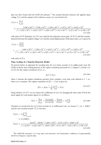
data was then found with the MATLAB software. The transfer-function between the applied input
voltage V x (t) and the output of the inductive sensor y(t) was found to be
Ys()
G 1 s() = -------------
V x s()
5.544 × 10 s – 7.528 × 10 s + 1.476 × 10 s – 4.571 × 10 s + 9.415 × 10 23
15 2
18
5 4
9 3
= ------------------------------------------------------------------------------------------------------------------------------------------------------------------------------------------------------------------------------
s + 1.255 × 10 s + 1.632 × 10 s + 1.855 × 10 s + 6.5 × 10 s + 6.25 × 10 s + 1.378 × 10 25
21
6
13 3
17 2
4 5
9 4
(23.134)
with units of V/V. Equation (23.135) was scaled by the inductive sensor gain (30 Å/V) and the transfer-
function between the applied voltage V x (t) and the actual displacement of the piezo-tube x p (t) is given by
X p s()
G 2 s() = -------------
V x s()
1.663 × 10 s – 2.258 × 10 s + 4.427 × 10 s – 1.371 × 10 s + 2.825 × 10 25
7 4
16 2
20
11 3
= ------------------------------------------------------------------------------------------------------------------------------------------------------------------------------------------------------------------------------
4 5
9 4
13 3
6
21
17 2
s + 1.255 × 10 s + 1.632 × 10 s + 1.855 × 10 s + 6.5 × 10 s + 6.25 × 10 s + 1.378 × 10 25
(23.135)
with units of Å/V.
Time Scaling of a Transfer-Function Model
We present below an approach for rescaling time for G 2 (s) from seconds [s] to milliseconds [ms]. We
briefly recall the time scaling property of the Laplace transform presented in [1, Chapter 3, section 1.4].
Let F(s) be the Laplace transform of f(t), i.e.,
L
ft() → Fs() (23.136)
ˆ
where L denotes the Laplace transform operator. Now, consider a new time scale defined as t = at ,
ˆ
where a is a constant. The Laplace transform of f(t) = f (at) is given by
L

1
s
ft() = fat() → -----F -- = F s() (23.137)
ˆ
ˆ
a a 
Using relation (23.137), we can reduce the coefficients of G 2 (s) by changing the time units of both the
input signal u(t) and output signal y(t) as follows:
(
(
Y s() Ys/a)/ a Ys/a) s
ˆ

ˆ
G s() = ----------- = ------------------------ = ---------------- = G -- (23.138)
(
(
U s() Us/a)/ a Us/a) a 
ˆ
Therefore, to rescale time for G 2 (s) from seconds [s] to millisecond [ms], we choose t ˆ = at = 0.001t
ˆ
and the new rescaled transfer G 2 (s) becomes
s
G 2 s() = 
ˆ
--
a 
G 2
a=0.001
= G 2 1000s)
(
1.371 ×
225.8s +
4.427 ×
2.825 ×
10 s +
5
4
4 2
3
7
10
10 s –
16.63s –
ˆ
G 2 s() = --------------------------------------------------------------------------------------------------------------------------------------------------------------------------------------------------------
6
4 3
3 4
5
6
5 2
s + 12.55s + 1.632 × 10 s + 1.855 × 10 s + 6.5 × 10 s + 6.25 × 10 s + 1.378 × 10 7
(23.139)
13
The MATLAB command invfreqs gives real numerator and denominator coefficients of experimentally
determined frequency response data.
©2002 CRC Press LLC