Page 737 - The Mechatronics Handbook

0066_Frame_C23 Page 45 Wednesday, January 9, 2002 1:56 PM

where C(t) is a q × n matrix and D(t) is a q × p matrix. In general, the matrices A(t), B(t), C(t), and D(t)
are time varying; however, in this chapter we will only consider the time-invariant case where A, B, C,
and D are constant matrices, then Eqs. (23.107) and (23.108) are called the linear time-invariant (LTI)
state and output equations, respectively. 3

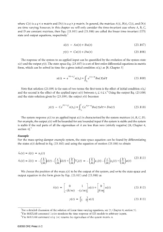
x ˙ t() = Ax t() + Bu t() (23.107)

yt() = Cx t() + Du t() (23.108)

The response of the system to an applied input can be quantified by the evolution of the system state
x(t) and the output y(t). The state-space Eq. (23.107) is a set of first order differential equations in matrix
form, which can be solved in time for a given initial condition x(t 0 ) as [8, Chapter 3]

(
At−t ) t At−t)
(
xt() = e 0 xt 0 + ∫ e Bu t()dt (23.109)
()
0 t
Note that solution (23.109) is the sum of two terms: the first term is the effect of initial condition x(t 0 )
4
and the second is the effect of the applied input u(t) between t 0 ≤ τ ≤ t. Using the output Eq. (23.108)
and the state solution given by (23.109), the output y(t) becomes

(
(
()
yt() = Ce At−t ) xt 0 + ∫ t Ce At−t) Bu t()dτ + Du t() (23.110)
0
t 0
The system response y(t) to an applied input u(t) is characterized by the system matrices (A, B, C, D).
For example, the output y(t) will be bounded for any bounded input if the system is stable and the system
is stable if the real parts of all the eigenvalues of A are less than zero (strictly negative) [8, Chapter 4,
5
section 4].
Example
For the mass-spring-damper example system, the state-space equation can be found by differentiating
the states x(t) defined in Eq. (23.102) and using the equation of motion (23.100) to obtain

x ˙ t() = z ˙ t() = x 2 t()
1
c
b
c
b
k
k
---- x 2 t() +
x ˙ t() = z ˙˙ t() = –    –    (23.111)
---- ut()
---- z ˙ t() +
---- V z t() =
---- x 1 t() –
---- zt() –






1
m
m
m
m
m
m
We choose the position of the mass z(t) to be the output of the system, and write the state-space and
output equation in the form given by Eqs. (23.107) and (23.108) as
0 1 0
x ˙ t() = xt() + ut() (23.112)
( – k/m) – ( c/m) b/m
yt() = 10 xt() (23.113)
3
For a detailed discussion of the solution of linear time-varying equations, see [7, Chapter 4, section 5].
4
The MATLAB command 1sim simulates the time response of LTI models to arbitrary inputs.
5
The MATLAB command eig (A)returns the eigenvalues of the system matrix A.
©2002 CRC Press LLC