Page 743 - The Mechatronics Handbook

0066_Frame_C23 Page 51 Wednesday, January 9, 2002 1:56 PM

ˆ
Note that the time unit of the input and output signal of G 2 (s) are now in milliseconds, not seconds!
ˆ
The coefficients of the numerator and denominator polynomials are smaller and this form (G 2 (s)) is less
prone to computational errors due to round off than the form G 2 (s), Eq. (23.135).
The State-Space Model
ˆ
The state-space realization for G 2 (s) expressed in controllable canonical form (Eqs. (23.132) and (23.133))
is given by the following:

– 12.55 – 1.632 × 10 3 – 1.855 × 10 4 – 6.50 × 10 5 – 6.25 × 10 6 – 1.378 × 10 7 1
1 0 0 0 0 0 0
x ˙ t() = 0 1 0 0 0 0 xt() + 0 ut()
0 0 1 0 0 0 0
0 0 0 1 0 0 0
0 0 0 0 1 0 0
(23.140)

7
yt() = [ 0 16.63 – 225.8 4.427 × 10 – 1.371 × 10 2.825 × 10 ]xt() (23.141)
5
4
The time unit for Eqs. (23.140) and (23.141) are milliseconds [ms]. If the initial state at t 0 is known,
along with the applied voltage V x (t) defined for t ≥ t 0 , the future behavior of the system, i.e., the state
x(t) and output y(t), can be determined from Eqs. (23.140) and (23.141), respectively.

Discrete-Time State-Space Modeling
Introduction
The study of discrete-time systems is important to the analysis and the design of modern mechatronics
systems where digital computers or small microprocessors are predominantly used to control systems.
Digital computers and microprocessors output or acquire information at discrete time instants. For
example, the input applied by a digital computer to actuate the piezo-tube changes at discrete time
instants. Similarly, the displacment of the piezo-tube can only be measured at specified time instants
using digital computers; therefore, in comparison to a continuous-time control system where the input
signals change continuously over time, the input of a discrete-time system changes once in a while. Such
discrete-time systems are studied next.
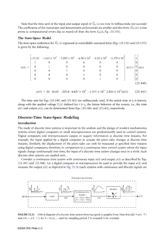
Consider a continuous-time system with continuous input u(t) and output y(t) as described by Eqs.
(23.107) and (23.108). Let a digital computer or microprocessor be used to provide the input u[k] and
measure the output y[k] as depicted in Fig. 23.24 (such systems with continuous and discrete signals are

Discrete-time System

u[k] u(t) y(t) Sampler y[k]
k t t k
0 1 2 3 4 5 . . . 0 1 2 3 4 5 . . . Continuous-time 0 1 2 3 4 5 . . . T 0 1 2 3 4 5 . . .
System
u[k] Hold . y[k]
u(t) x(t) = Ax(t) + Bu(t) y(t)
y(t) = Cx(t) + Du(t)

⋅
FIGURE 23.24 A block diagram of a discrete-time system showing signals in graphic from. Note that u[k] = u(kT )
and y[k] = y(kT⋅ ), for k = 0,1,2,…, and the sampling period T is assumed to be constant.

©2002 CRC Press LLC