Page 747 - The Mechatronics Handbook

0066_Frame_C23 Page 55 Wednesday, January 9, 2002 1:56 PM

b
m
k
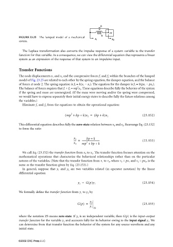
FIGURE 23.25 The lumped model of a mechanical
x 1 x
system. 2
The Laplace transformation also converts the impulse response of a system variable to the transfer
function for that variable. As a consequence, we can view the differential equation that represents a linear
system as an expression of the response of that system to an impulsive input.

Transfer Functions

The node displacements x 1 and x 2 and the compressive forces f 1 and f 2 within the branches of the lumped
model of Fig. 23.25 are related to each other by the spring equation, the damper equation, and the balance
of forces at node 2. The spring equation is f 2 = k(x 1 − x 2 ). The equation for the damper is f 1 = b(px 1 − px 2 ).
2
The balance of forces requires that f 1 + f 2 = mp x 2 . These equations describe fully the behavior of the system
if the spring and mass are unenergized. (If the mass were moving and/or the spring were compressed,
we would have to express separately their initial energy states to describe fully the future relations among
the variables.)
Eliminate f 1 and f 2 from the equations to obtain the operational equation:

( mp + bp + k)x 2 = ( bp + k)x 1 (23.152)
2
This differential equation describes fully the zero-state relation between x 1 and x 2 . Rearrange Eq. (23.152)
to form the ratio

bp +
k
---- = ------------------------------- (23.153)
x 2
mp + bp +
2
x 1 k
We call Eq. (23.152) the transfer function from x 1 to x 2 . The transfer function focuses attention on the
mathematical operations that characterize the behavioral relationships rather than on the particular
natures of the variables. (Note that the transfer function from v 1 to v 2 , where v 1 = px 1 and v 2 = px 2 , is the
same as the transfer function given by Eq. (23.153).)
In general, suppose that y 1 and y 2 are two variables related (in operator notation) by the linear
differential equation

y 2 = Gp()y 1 (23.154)

We formally define the transfer function from y 1 to y 2 by

y 2
Gp() = ---- (23.155)
y 1
ZS
where the notation ZS means zero state. If y 1 is an independent variable, then G(p) is the input–output
transfer function for the variable y 2 and accounts fully for its behavior owing to the input signal y 1 . We
can determine from that transfer function the behavior of the system for any source waveform and any
initial state.

©2002 CRC Press LLC