Page 750 - The Mechatronics Handbook

0066_Frame_C23 Page 58 Wednesday, January 9, 2002 1:56 PM

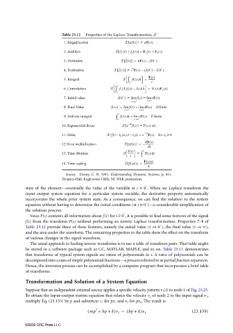
Table 23.12 Properties of the Laplace Transformation,
[
1. Magnification af t()] = aF s()
[
2. Addition f 1 t() + f 2 t()] = F 1 s() + F 2 s()
−
˙
[
3. Derivative f t()] = sF s() – f 0()
−
−
2
˙˙
[
4. Derivatives f t()] = s F s() – sf 0() – ˙ f 0()
t F s()
5. Integral − ∫ f t() dt = ----------
0 s
t
(
6. Convolution − ∫ f 1 l()f 2 t – l) dl = F 1 s()F 2 s()
0
+
(
7. Initial value f 0 ) = lim ft() = lim sF s()
+ s→∞
t→0
8. Final Value f ∞() = lim ft() = lim sF s() if finite
t→∞ s→0
∞
9. Definite integral ∫ f t() dt = lim sF s() if finite
0 s → 0
(
[
10. Exponential decay e – at ft()] = F s + a)
[
(
(
11. Delay ft – )u s t – )] = e – t 0 s F s() for t 0 ≥ 0
t 0
t 0
dF s()
[
12.Time multiplication tf t()] = – -------------
ds
ft() ∞
13. Time division -------- = ∫ F s()ds
t s
(
F s/a)
[
14. Time scaling fat()] = ---------------
a
Source: Dorny, C. N. 1993. Understanding Dynamic Systems, p. 413.
Prentice-Hall, Englewood Cliffs, NJ. With permission.
−
state of the element—essentially the value of the variable at t = 0 . When we Laplace transform the
input–output system equation for a particular system variable, the derivative property automatically
incorporates the whole prior system state. As a consequence, we can find the solution to the system
+
equation without having to determine the initial conditions (at t = 0 )—a considerable simplification of
the solution process.
−
Since F(s) contains all information about f(t) for t ≥ 0 , it is possible to find some features of the signal
f(t) from the transform F(s) without performing an inverse Laplace transformation. Properties 7–9 of
+
Table 23.12 provide three of these features, namely the initial value (t → 0 ), the final value (t → ∞),
and the area under the waveform. The remaining properties in the table show the effect on the transform
of various changes in the signal waveform.
The usual approach to finding inverse transforms is to use a table of transform pairs. That table might
be stored in a software package such as CC, MATLAB, MAPLE, and so on. Table 23.11 demonstrates
that transforms of typical system signals are ratios of polynomials in s. A ratio of polynomials can be
decomposed into a sum of simple polynomial fractions—a process referred to as partial fraction expansion.
Hence, the inversion process can be accomplished by a computer program that incorporates a brief table
of transforms.
Transformation and Solution of a System Equation
Suppose that an independent external source applies a specific velocity pattern v 1 (t) to node 1 of Fig. 23.25.
To obtain the input–output system equation that relates the velocity v 2 of node 2 to the input signal v 1 ,
multiply Eq. (23.153) by p and substitute v 1 for px 1 and v 2 for px 2 . The result is
2
( mp + bp + k)v 2 = ( bp + k)v 1 (23.159)
©2002 CRC Press LLC