Page 755 - The Mechatronics Handbook

For continuous-time systems

dx
------ = Fx t(), u t(), t) (24.1)
(
dt
(
y t() = Gx t(), u t(), t) (24.2)
where u(t) is the system input vector and y(t) is an output vector.
For discrete-time systems

x t + 1] = F d x t[], u t[], t( ) (24.3)
[
y t[] = G d x t[], u t[], t( ) (24.4)
Similarly to the continuous-time case, u[t] is the system input vector and y[t] is an output vector.
Note that throughout this chapter we will use the symbol t to denote continuous and discrete time, but
the difference will be made on using [ and ] to enclose the argument in the discrete-time case, when t Π.
To obtain a first glimpse at the concepts underlying the state space approach, we consider the following
example.
Example 24.1
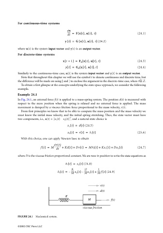
In Fig. 24.1, an external force f(t) is applied to a mass-spring system. The position d(t) is measured with
respect to the mass position when the spring is relaxed and no external force is applied. The mass
movement is damped by a viscous friction force proportional to the mass velocity, v(t).
From first principles we know that to be able to compute the mass position and the mass velocity we
must know the initial mass velocity, and the initial spring stretching. Thus, the state vector must have
T
two components, i.e., x(t) = [x 1 (t) x 2 (t)] , and a natural state choice is
x 1 t() = dt() (24.5)

x 2 t() = vt() = x ˙ 1 t() (25.6)
With this choice, one can apply Newton laws to obtain
dvt()
f t() = M ------------ + Kd t() + Dv t() = Mx ˙ 2 t() + Kx 1 t() + Dx 2 t() (24.7)
dt

where D is the viscous friction proportional constant. We are now in position to write the state equations as

x ˙ 1 t() = x 2 t() (24.8)
K D 1
x ˙ 2 t() = – ----- x 1 t() – ----- x ----- ft() (24.9)
M 2 t() +
M
M
v(t)
d(t)
K
M f(t)

viscous friction

FIGURE 24.1 Mechanical system.

©2002 CRC Press LLC