Page 759 - The Mechatronics Handbook

0066_Frame_C24 Page 7 Thursday, January 10, 2002 3:43 PM

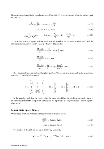
Hence, the state in equilibrium can be computed from (24.32) to (24.34), setting all the derivatives equal
to zero, i.e.,

R
−---x 1Q + 1 0 ⇒ x 1Q = E Q (24.35)
---E Q =
------
L L R
– x 3Q = 0 ⇒ x 3Q = 0 (24.36)
K 1 K 1 K 1 E Q
-----------------------------x 1Q – g = 0 ⇒ x 2Q = -------x 1Q – K 2 = ------------ – K 2 (24.37)
(
mx 2Q + K 2 ) mg mgR
The setting now is adequate to build the linearized model in the incremental input ∆e(t) and the
T
incremental state ∆x(t) = [∆x 1 (t) ∆x 2 (t) ∆x 3 (t)] . The result is
d∆ x 1 t() R 1
-------------------- = – ---∆ x 1 t() + ---∆et() (24.38)
dt L L

d∆ x 2 t()
-------------------- = – ∆ x 3 t() (24.39)
dt

d∆ x 3 t() Rg Rmg 2
-------------------- = ------∆ x 1 t() – -------------∆ x 2 t() (24.40)
dt E Q K 1 E Q

If we define as the system output, the sphere position h(t), we can then compare the above equations
with (24.23) and (24.24) to obtain

R
– --- 0 0 1
L --- 0
A = 0 0 – 1 , B = L , C = 1 , D = 0 (24.41)
0
Rg Rmg 2 0
------ – -------------- 0 0
E Q K E
1 Q
In the sequel we will drop the prefix ∆, but the reader should bear in mind that the model above is
linear in the incremental components of the state, the inputs and the outputs around a chosen equilib-
rium point.

Linear State Space Models
Our starting point is now the linear time invariant state space model

dx t()
------------- = Ax t() + Bu t() (24.42)
dt
y t() = Cx t() + Du t() (24.43)

The solution to Eq. (24.42), subject to x(t o ) = x o , is given by

(
(
x t() = e A t−t ) x o + ∫ t e A t−t ) Bu t() t ∀ t ≥ t o (24.44)
o
d
o t
©2002 CRC Press LLC