Page 758 - The Mechatronics Handbook

0066_Frame_C24 Page 6 Thursday, January 10, 2002 3:43 PM

i(t)
R +
L e(t)

h(t) f(t) v(t)

mg

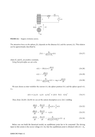
FIGURE 24.2 Magnetic levitation system.

The attraction force on the sphere, f(t), depends on the distance h(t) and the current, i(t). This relation
can be approximately described by

ft() = ----------------------it() (24.27)
K 1
ht() + K 2
where K 1 and K 2 are positive constants.
Using first principles we can write

di t()
et() = Ri t() + L ----------- (24.28)
dt
dh t()
vt() = – ------------- (24.29)
dt
dv t()
ft() = ----------------------it() = mg + m------------ (24.30)
K 1
ht() + K 2 dt
We next choose as state variables: the current i(t), the sphere position h(t), and the sphere speed v(t),
i.e.,

T
xt() = [ x 1 t() x 2 t() x 3 t()] = [ it() ht() vt()] T (24.31)
Then, from (24.28)–(24.30) we can set the system description as in (24.1) yielding

di t() dx 1 t() R 1 (24.32)
---x 1 t() +
----------- =
--------------- =
---et()
dt dt – L L
dh t() dx 2 t()
------------- = --------------- = – x 3 t() (24.33)
dt dt
dv t() dx 3 t() ---------------------------------x 1 t() g– (24.34)
--------------- =
------------ =
K 1
(
dt dt mx 2 t() + K 2 )
Before one can build the linearized model, an equilibrium point has to be computed. The driving
input in this system is the source voltage e(t). Say that the equilibrium point is obtained with e(t) = E Q .

©2002 CRC Press LLC