Page 763 - The Mechatronics Handbook

0066_Frame_C24 Page 11 Thursday, January 10, 2002 3:44 PM

close to the resonant frequency. For example, if a system has eigenvalues λ 1,2 = −0.05 ± j, i.e., the resonant
frequency is 1 rad/s and, additionally, one of the input components is a sine wave of frequency 0.9 rad/s,
then the system output exhibits a very large (forced) oscillation with amplitude initially growing almost
linearly and later, stabilizing to a constant value. In real situations this phenomenon may destroy the
system (recall the Tacoma bridge case).

State Similarity Transformation
We have already said that the choice of state variables is nonunique. Say that we have a system with input
n
u(t), output y(t), and two different choices of state vectors: x(t) ∈ with an associated 4-tuple (A, B,
,
,,
n
x
C, D), and (t) ∈ with an associated 4-tuple (ABCD ). Then there exists a nonsingular matrix
n×n
T ∈ such that
–
x t() = Tx t() ⇔ x t() = T x t() (24.58)
1
This leads to the following equivalences:
A = TAT , B = TB, C = CT – 1 (24.59)
1
–
Different choices of state variables may or may not respond to different phenomenological approaches
to the system analysis. Sometimes it is just a question of mathematical simplicity, as we shall see in section
24.6. In other occasions, the decision is made considering relative facility to measure certain system variables.
However, what is important is that, no matter which state description is chosen, certain fundamental
system characteristics do not change. They are related to the fact that the system eigenvalues are invariant
with respect to similarity transformations, since
(
(
–
1
1
–
1
–
(
(
det lIA) = det lTT – TAT ) = det T()det lIA)det T ) (24.60)
–
–
= det lIA) (24.61)
(
–
Hence, stability, nature of the unforced response, and speed of response are invariants with respect to
similarity transformations.
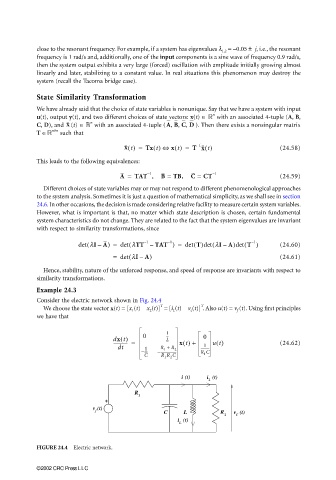
Example 24.3
Consider the electric network shown in Fig. 24.4
T
T
We choose the state vector x(t) = [x 1 (t) x 2 (t)] = [i L (t) v c (t)] . Also u(t) = v f (t). Using first principles
we have that
1
dx t() 0 --- L x t() + 0 ut() (24.62)
------------- =
1
dt 1 R + R 2 ----------
1
– --- – ------------------ R C
C R R C 1
2
1
i (t) i (t)
2
R
1
+
v (t)
f C L R v (t)
2 C
i (t)
L
FIGURE 24.4 Electric network.
©2002 CRC Press LLC