Page 767 - The Mechatronics Handbook

0066_Frame_C24 Page 15 Thursday, January 10, 2002 3:44 PM

Linearization of Discrete Time Systems
The discrete time equivalents to (24.3) and (24.4) are given by the nonlinear equations

x t + 1] = F d x t[], u t[]) (24.82)
[
(
y t[] = G d x t[], u t[]( ) (24.83)

The linearization of models for discrete time systems follows along the same lines to that for continuous
ones. Consider firstly an equilibrium point given by {x Q , u Q , y Q }:

x Q = F d x Q , u Q ) (24.84)
(
(
y Q = G d x Q , u Q ) (24.85)

Note that an equilibrium point is defined by a set of constant values of the state and constant values
of the input which satisfy (24.82) and (24.83). This yields a constant system output. The discrete model
can then be linearized around this equilibrium point. Defining
∆x t[] = x t[] x Q ,– ∆u t[] = u t[] u Q , ∆y t[] = y t[] y Q (24.86)
–
–
we have the state space model
[
∆x t + 1] = A d ∆x t[] + B d ∆u t[] (24.87)
∆y t[] = C d ∆x t[] + D d ∆u t[] (24.88)

where

A d = ∂F d x=x , B d = ∂F d x=x , C d = ∂ G d x=x , D d = ∂G d x=x (24.89)
----------
--------
---------
--------
∂ x u=u ∂ u u=u Q Q ∂ x u=u ∂ u u=u Q Q
Q
Q
Q
Q
Sampled Data Systems
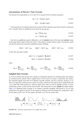
As we have already said, discrete time models are frequently obtained by sampling inputs and outputs
in continuous-time systems. When a digital device is to be used to act upon a continuous-time system,
the command signals need only to be defined at specific instants, and not at all time. However, to be
able to act upon the continuous-time system, we need a continuous-time signal. This is usually built with
a zero order hold, which generates a staircase signal. Also, when we want to digitally measure a system
variable this is done at some specific time instants. This means that we must sample the output signals.
Figure 24.5 illustrates these concepts. If we assume a periodic sampling, with period ∆, we are only
interested in the signals at time k∆. In the sequel we will drop ∆ from the arguments, using u(k∆) = u[t]
for the input, y(k∆) = y[t] for the output, and x(k∆) = x[t] for the system state.

Continuous
Hold Sample
Time System
u[t] u (t) y (t) y[t]
s
FIGURE 24.5 Schematic representation of a sampled data system.

©2002 CRC Press LLC