Page 769 - The Mechatronics Handbook

0066_Frame_C24 Page 17 Thursday, January 10, 2002 3:44 PM

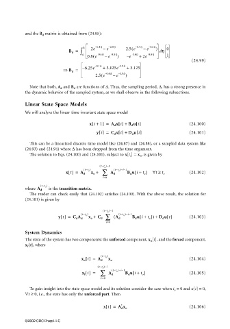
and the B d matrix is obtained from (24.95):

∆ – 0.4h – 0.8h ( – 0.4h – 0.8h )
B d = ∫ 2e – e 2.5 e – e d h 0
0 0.8 e ( – 0.4h – e – 0.8h ) e – – 0.4h + 2e – 0.8h 1
(24.99)

⇒ B d = – 6.25e – 0.4∆ + 3.125e – 0.8∆ + 3.125
2.5 e ( – 0.4∆ – e – 0.8∆ )

Note that both, A d and B d are functions of ∆. Thus, the sampling period, ∆, has a strong presence in
the dynamic behavior of the sampled system, as we shall observe in the following subsections.

Linear State Space Models

We will analyze the linear time invariant state space model
[
x t + 1] = A d x t[] + B d u t[] (24.100)
y t[] = C d x t[] + D d u t[] (24.101)

This can be a linearized discrete time model like (24.87) and (24.88), or a sampled data system like
(24.93) and (24.94) where ∆ has been dropped from the time argument.
The solution to Eqs. (24.100) and (24.101), subject to x[t o ] = x o , is given by

( t−t )−1
o
x t[] = A d ( t−t ) x o + ∑ A d ( t−t )−i−1 B d u i + ] ∀ t ≥ t o (24.102)
[
o
o
t o
i=0
( t−t )
o
where A d is the transition matrix.
The reader can check easily that (24.102) satisfies (24.100). With the above result, the solution for
(24.101) is given by
( t−t )−1
o
y t[] = C d A ( t−t ) x o + C d ∑ ( ( t−t )−i−1 B d u i + ]) + D d u t[] (24.103)
[
o
o
d A d t o
i=0
System Dynamics
The state of the system has two components: the unforced component, x u [t], and the forced component,
x f [t], where
x u t[] = A d ( t−t ) x o (24.104)
o
( t−t )−1
o
x f t[] = ∑ A d ( t−t )−i−1 B d u i + ] (24.105)
[
o
t o
t =0
To gain insight into the state space model and its solution consider the case when t o = 0 and u[t] = 0,
∀ t ≥ 0 , i.e., the state has only the unforced part. Then
x t[] = A d x o (24.106)
t

©2002 CRC Press LLC