Page 773 - The Mechatronics Handbook

0066_Frame_C24 Page 21 Thursday, January 10, 2002 3:45 PM

5
y[t]
u[t]
0

-5
0 5 10 15 20 25 30 35 40
discrete time t
3
y[t]
2 u[t]
1
0
-1
-2
-3
0 5 10 15 20 25 30 35 40
discrete time t

FIGURE 24.7 Resonant effect in the system output.

Sampling time ∆ = 0.5
1

x 1 [t] 0.5

0
0 2 4 6 8 10 12 14 16 18 20
Sampling time ∆ = 1
1
x 1 [t] 0.5

0
0 2 4 6 8 10 12 14 16 18 20
Sampling time ∆ = 2
1

x 1 [t] 0.5

0
0 2 4 6 8 10 12 14 16 18 20
discrete time t
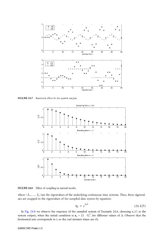
FIGURE 24.8 Effect of sampling in natural modes.

}are the eigenvalues of the underlying continuous-time systems. Then, these eigenval-
where {l 1 ,…, l n
ues are mapped to the eigenvalues of the sampled-data system by equation:
h = e l ∆ (24.125)

In Fig. 24.8 we observe the response of the sampled system of Example 24.6, choosing x 1 [t] as the
T
system output, when the initial condition is x o = [1 0] , for different values of ∆. Observe that the
horizontal axis corresponds to t, so the real instants times are t∆.

©2002 CRC Press LLC