Page 777 - The Mechatronics Handbook

0066_Frame_C24 Page 25 Thursday, January 10, 2002 3:45 PM

and the composite system output is y(t) = y 1 (t). We thus obtain

x ˙ 1 t() x 1 t()
= A 1 B 1 C 2 + B 1 D 2 u t() (24.146)
x ˙ 2 t() 0 A 2 x 2 t() B 2

x 1 t()
y t() = [ C 1 D 1 C 2 ] + [ D 1 D ] u t() (24.147)
x 2 t() 2

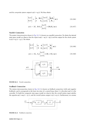
Parallel Connection
The system interconnection shown in Fig. 24.11 is known as a parallel connection. To obtain the desired
state space model we observe that the input is u(t) = u 1 (t) = u 2 (t) and the output for the whole system
is y(t) = y 1 (t) + y 2 (t). We obtain

x ˙ 1 t() x 1 t()
= A 1 0 + B 1 u t() (24.148)
x ˙ 2 t() 0 A 2 x 2 t() B 2

x 1 t()
y t() = [ C 1 C 2 ] + [ D 1 + D ] u t() (24.149)
x 2 t() 2

u (t) y (t)
1 1
x (t)
1
u(t) + y(t)
+
x (t)
u (t) 2 y (t)
2 2

FIGURE 24.11 Parallel connection.

Feedback Connection
The system interconnection shown in Fig. 24.12 is known as feedback connection (with unit negative
feedback), and it corresponds to the basic structure of a control loop, where S 1 is the plant and S 2 is the
controller. To build the composite state space model we observe that the overall system input satisfies
the equation u(t) = u 2 (t) + y 1 (t), and the overall system output is y(t) = y 1 (t). Furthermore, we assume

u(t) u (t) y (t) y (t) y(t)
2 x (t) 2 x (t) 1
+ 2 1
− u (t)
1

FIGURE 24.12 Feedback connection.

©2002 CRC Press LLC