Page 774 - The Mechatronics Handbook

0066_Frame_C24 Page 22 Thursday, January 10, 2002 3:45 PM

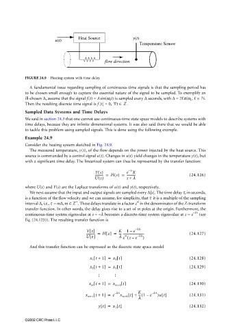
Heat Source y(t)
u(t)
Temperature Sensor

flow direction

FIGURE 24.9 Heating system with time delay.

A fundamental issue regarding sampling of continuous-time signals is that the sampling period has
to be chosen small enough to capture the essential nature of the signal to be sampled. To exemplify an
ill-chosen ∆, assume that the signal f(t) = Asin(w o t) is sampled every ∆ seconds, with ∆ = 2 p/w o , ∈ .
Then the resulting discrete time signal is f [t] = 0, t∀ ∈ .
Sampled Data Systems and Time Delays
We said in section 24.3 that one cannot use continuous-time state space models to describe systems with
time delays, because they are infinite dimensional systems. It was also said there that we would be able
to tackle this problem using sampled signals. This is done using the following example.
Example 24.9
Consider the heating system sketched in Fig. 24.9.
The measured temperature, y(t), of the flow depends on the power injected by the heat source. This
source is commanded by a control signal u(t). Changes in u(t) yield changes in the temperature y(t), but
with a significant time delay. The linearized system can thus be represented by the transfer function:

Ys() e K
–
ts
----------- = Hs() = ----------- (24.126)
Us() s + l
where U(s) and Y(s) are the Laplace transforms of u(t) and y(t), respectively.
We next assume that the input and output signals are sampled every ∆[s]. The time delay t, in seconds,
is a function of the flow velocity and we can assume, for simplicity, that t it is a multiple of the sampling
interval ∆, i.e., t = m∆, m ∈ + . These delays translate in a factor z in the denominator of the Z-transform
m
transfer function. In other words, the delay gives rise to a set of m poles at the origin. Furthermore, the
−l∆
continuous-time system eigenvalue at s = −l becomes a discrete-time system eigenvalue at z = e (see
Eq. (24.125)). The resulting transfer function is

Yz[] K 1 e – l∆
–
----------- = Hz[] = --- ---------------------------- (24.127)
Uz[] l z ze – l∆ )
(
m
–
And this transfer function can be expressed as the discrete state space model
[
x 1 t + 1] = x 2 t[] (24.128)
x 2 t +[ 1] = x 3 t[] (24.129)

x m t +[ 1] = x m+1 t[] (24.130)

[
x m+1 t + 1] = e – l∆ x m+1 t[] + K ( – – l∆ )ut[] (24.131)
--- 1 e
l
yt[] = x 1 t[] (24.132)

©2002 CRC Press LLC