Page 776 - The Mechatronics Handbook

0066_Frame_C24 Page 24 Thursday, January 10, 2002 3:45 PM

One way to obtain the state space model is to use the same method proposed in section “State Space and
Transfer Functions,” applying Zeta transformation instead of Laplace transformation, and using the fact that

Fz[] = Z ft[]{ } ⇔ zF z[] = Z ft +[{ 1]} (24.138)

Example 24.10
The transfer function of a system is given by
2
1.8z +
2z – +
z
1
0.04
Hz[] = ----------------------------------------- = ------------------------------------ + 2 (24.139)
(
( z 0.8) z 0.6) z – 1.4z + 0.48
–
2
–
Then a minimal realization for this system is
A d = 0 1 , B d = 0 (24.140)
– 0.48 – 1.4 1
C d = [ 0.04 1.8], D d = 2 (24.141)
In discrete-time models it also happens that the system transfer function is invariant with respect
to state similarity transformations.

24.5 State Space Models for Interconnected Systems

To build state space models for complex systems it is sometimes useful (and possible) to describe them
as the interconnection of simpler systems. That interconnection is usually a combination of three basic
interconnection structures: series, parallel, and feedback. In those three basic cases our aim is to obtain
a state space model for the composite system.
In the following analysis we will use two systems, which are defined by
dx 1 t()
System 1: --------------- = A 1 x 1 t() + B 1 u 1 t() (24.142)
dt
y 1 t() = C 1 x 1 t() + D 1 u 1 t() (24.143)

dx 2 t()
System 2: --------------- = A 2 x 2 t() + B 2 u 2 t() (24.144)
dt
y 2 t() = C 2 x 2 t() + D 2 u 2 t() (24.145)

Series Connection
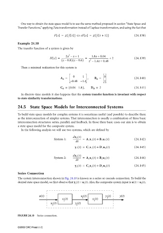
The system interconnection shown in Fig. 24.10 is known as a series or cascade connection. To build the
desired state space model, we first observe that y 2 (t) = u 1 (t). Also, the composite system input is u(t) = u 2 (t),

u(t) u (t) y (t) y(t)
x (t) 1 x (t) 1
2 1
u (t) y (t)
2 2

FIGURE 24.10 Series connection.

©2002 CRC Press LLC